KL-minimizing Sparse GMRF Approximations to Gaussian Processes

Introduction

Gaussian processes (GPs) are a powerful tool for probabilistic modeling, but they suffer from cubic scaling in the number of data points due to the need to invert dense covariance matrices. When working with spatial or temporal data, we can often approximate a GP as a Gaussian Markov Random Field (GMRF), which has a sparse precision matrix and thus enables much more efficient computation.

In this tutorial, we demonstrate how to approximate a GP defined by a kernel function using a sparse GMRF via the Kullback-Leibler (KL) divergence minimizing Cholesky approximation. This approach:

• Takes a kernel matrix (covariance matrix) and input locations

• Computes a sparse approximate Cholesky factorization

• Returns a GMRF that approximates the original GP

We'll demonstrate this by:

1. Creating a GP with a Matern 3/2 kernel on a 2D spatial grid

2. Approximating it as a sparse GMRF

3. Conditioning on a handful of observations

4. Visualizing the posterior to validate the Matern spatial correlation structure

The algorithm presented here is described in detail in [3].

Setup

Let's begin by loading the necessary packages:

using GaussianMarkovRandomFields
using KernelFunctions
using LinearAlgebra
using SparseArrays
using Random
using Distributions
using CairoMakie

Random.seed!(123)

Random.TaskLocalRNG()

Creating a spatial grid

We'll work with a 2D spatial grid. Let's create a 30 x 30 grid of points in the unit square:

n_x = 30
n_y = 30
xs = range(0, 1, length = n_x)
ys = range(0, 1, length = n_y)

0.0:0.034482758620689655:1.0

Next, we turn the grid points into a matrix where each column is a point [x, y].

points = [(x, y) for x in xs, y in ys]
X = hcat([[p[1], p[2]] for p in vec(points)]...)

n_points = size(X, 2)
println("Created grid with $n_points points")

Created grid with 900 points

Defining a Gaussian Process with a Matern kernel

We'll use a Matern 3/2 kernel, which is a popular choice for spatial modeling. The Matern 3/2 kernel has the form:

$$k(r)={\sigma }^2(1+\frac{\sqrt{3}r}{\ell })\exp (-\frac{\sqrt{3}r}{\ell })$$

where $r$ is the distance between points, $\ell$ is the length scale, and ${\sigma }^2$ is the variance.

Let's define the kernel with length scale l = 0.3 and variance sigma2 = 1.0.

l = 0.3
sigma2 = 1.0
kernel = sigma2 * with_lengthscale(Matern32Kernel(), l)

Matern 3/2 Kernel (metric = Distances.Euclidean(0.0))
	- Scale Transform (s = 3.3333333333333335)
	- σ² = 1.0

Now compute the kernel matrix (covariance matrix) at all grid points.

K = kernelmatrix(kernel, X, obsdim = 2)

println("Kernel matrix size: ", size(K))
println("Kernel matrix is dense with $(length(K)) entries")

Kernel matrix size: (900, 900)
Kernel matrix is dense with 810000 entries

Approximating the GP evaluation with a sparse GMRF

Now we use the KL-divergence minimizing sparse Cholesky approximation to create a GMRF that approximates the evaluation of this GP. The key parameters are:

• ρ (rho): Controls the radius of the neighborhood used to determine the sparsity pattern. Larger values result in denser (and more accurate) approximations.

• λ (lambda): Controls supernodal clustering for improved performance. Default is 1.5, which groups nearby columns together for better cache efficiency. Set to nothing for standard column-by-column factorization.

rho = 2.0  # Neighborhood radius parameter
gmrf = approximate_gmrf_kl(K, X; ρ = rho)  # Uses supernodal factorization by default (λ=1.5)

Q = precision_matrix(gmrf)
println("GMRF precision matrix size: ", size(Q))
println("Number of non-zeros in precision matrix: ", nnz(Q))
println("Sparsity: ", round(100 * (1 - nnz(Q) / length(Q)), digits = 2), "%")

GMRF precision matrix size: (900, 900)
Number of non-zeros in precision matrix: 35156
Sparsity: 95.66%

Conditioning on observations

To validate that the GMRF approximation captures the Matern spatial correlation, we'll condition on a small number of observations at different locations. We'll place 3 observation points with specific values to see the spatial correlation structure emerge.

Let's select three observation locations at different positions in the grid.

obs_locs = [
    (0.25, 0.25),  # Bottom-left quadrant
    (0.75, 0.5),   # Right side, middle
    (0.5, 0.75),    # Top, center
]

3-element Vector{Tuple{Float64, Float64}}:
 (0.25, 0.25)
 (0.75, 0.5)
 (0.5, 0.75)

We need to find the grid indices closest to these locations.

obs_indices = Int[]
for (x_obs, y_obs) in obs_locs
    dists = [sqrt((X[1, i] - x_obs)^2 + (X[2, i] - y_obs)^2) for i in 1:n_points]
    push!(obs_indices, argmin(dists))
end

Set the observation values:

y_obs = [1.0, -1.0, 0.5]  # Different values at each location

3-element Vector{Float64}:
  1.0
 -1.0
  0.5

... and the observation noise:

obs_noise_std = 0.05

println("Observations at $(length(obs_indices)) locations:")
for (i, idx) in enumerate(obs_indices)
    println("  Point $(i): ($(round(X[1, idx], digits = 2)), $(round(X[2, idx], digits = 2))) = $(y_obs[i])")
end

Observations at 3 locations:
  Point 1: (0.24, 0.24) = 1.0
  Point 2: (0.76, 0.48) = -1.0
  Point 3: (0.48, 0.76) = 0.5

Now we condition the GMRF on the observations using linear_condition.

Create observation matrix (selects observed locations):

n_obs = length(obs_indices)
A = sparse(1:n_obs, obs_indices, ones(n_obs), n_obs, n_points)

3×900 SparseArrays.SparseMatrixCSC{Float64, Int64} with 3 stored entries:
⎡⠀⠀⠀⠀⠀⠀⠀⠀⠀⠈⠀⠀⠀⠀⠀⠀⠀⠀⠀⢀⠀⠀⠀⠀⠀⠀⠀⠀⠀⠀⠀⠀⠀⠀⠀⠀⠀⠀⠀⠀⎤
⎣⠀⠀⠀⠀⠀⠀⠀⠀⠀⠀⠀⠀⠀⠀⠀⠀⠀⠀⠀⠀⠀⠀⠀⠀⠀⠀⠀⠀⠀⢀⠀⠀⠀⠀⠀⠀⠀⠀⠀⠀⎦

Observation precision (inverse variance):

Q_eps = sparse(Diagonal(fill(1.0 / obs_noise_std^2, n_obs)))

3×3 SparseArrays.SparseMatrixCSC{Float64, Int64} with 3 stored entries:
 400.0     ⋅      ⋅ 
    ⋅   400.0     ⋅ 
    ⋅      ⋅   400.0

Compute the posterior:

posterior = linear_condition(gmrf; A = A, Q_ϵ = Q_eps, y = y_obs)

GMRF{Float64} with 900 variables
  Algorithm: LinearSolve.CHOLMODFactorization{Nothing}
  Mean: [0.4369443160792732, 0.46675903368586913, 0.4960127462521874, ..., -0.09260099682270781, -0.09927625478684732, -0.10242438007738269]
  Q_sqrt: not available

Extract the posterior mean and standard deviation:

posterior_mean = mean(posterior)
posterior_std = std(posterior)
posterior_mean[1:5], posterior_std[1:5]

([0.4369443160792732, 0.46675903368586913, 0.4960127462521874, 0.5296468485786933, 0.5497336926959444], [0.9093108101875973, 0.891117191617424, 0.8715392379842478, 0.8475621451360154, 0.8266549921705657])

Visualization

Let's visualize the posterior distribution to validate that it captures the Matern spatial correlation structure.

posterior_mean_grid = reshape(posterior_mean, n_x, n_y)
posterior_std_grid = reshape(posterior_std, n_x, n_y)
fig = Figure(size = (1000, 400))

ax1 = Axis(fig[1, 1], title = "Posterior Mean", xlabel = "x", ylabel = "y")
hm1 = heatmap!(ax1, xs, ys, posterior_mean_grid, colormap = :RdBu)
scatter!(
    ax1, X[1, obs_indices], X[2, obs_indices],
    color = :black, markersize = 12, marker = :circle, strokewidth = 2, strokecolor = :white
)
Colorbar(fig[1, 2], hm1, label = "Value")

ax2 = Axis(fig[1, 3], title = "Posterior Std. Deviation", xlabel = "x", ylabel = "y")
hm2 = heatmap!(ax2, xs, ys, posterior_std_grid, colormap = :inferno)
scatter!(
    ax2, X[1, obs_indices], X[2, obs_indices],
    color = :cyan, markersize = 12, marker = :circle, strokewidth = 2, strokecolor = :black
)
Colorbar(fig[1, 4], hm2, label = "Std. Dev.")

fig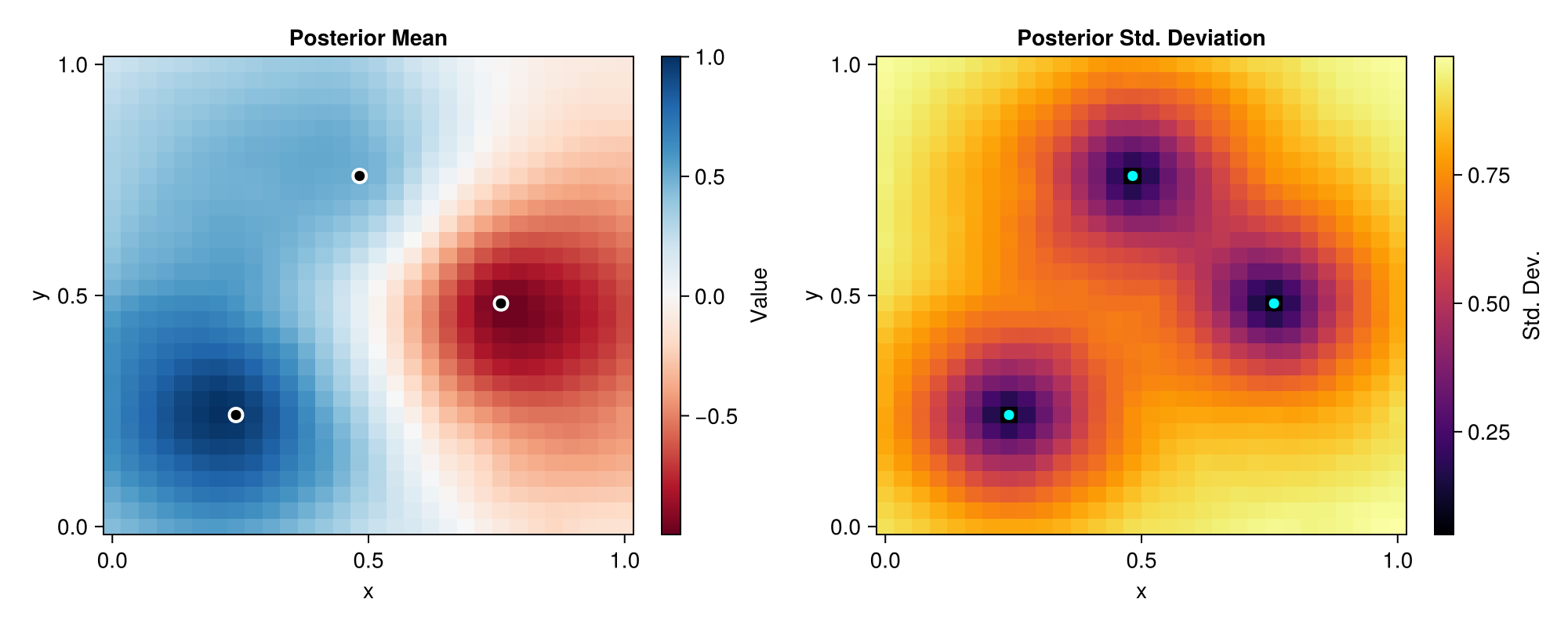

The posterior mean shows smooth spatial correlation characteristic of the Matern 3/2 kernel. Notice how the influence of each observation decreases with distance according to the length scale. The posterior standard deviation is minimal at observation locations and increases with distance, exhibiting the expected spatial correlation structure of a Matern process.

Effect of the ρ parameter

The ρ parameter controls the sparsity-accuracy tradeoff. Larger values include more neighbors in the sparsity pattern, leading to better approximations but with less sparsity. Let's compare the approximation quality for different ρ values.

rho_values = [2.0, 2.5, 3.0]
posteriors = Dict()
sparsities = Dict()

for rho_val in rho_values
    gmrf_temp = approximate_gmrf_kl(K, X; ρ = rho_val)
    Q_temp = precision_matrix(gmrf_temp)
    sparsities[rho_val] = 100 * (1 - nnz(Q_temp) / length(Q_temp))

    posterior_temp = linear_condition(gmrf_temp; A = A, Q_ϵ = Q_eps, y = y_obs)
    posteriors[rho_val] = posterior_temp
end

fig_comparison = Figure(size = (1200, 900))

for (idx, rho_val) in enumerate(rho_values)
    post = posteriors[rho_val]
    mean_grid = reshape(mean(post), n_x, n_y)
    std_grid = reshape(std(post), n_x, n_y)

    ax_mean = Axis(
        fig_comparison[idx, 1],
        title = "ρ = $(rho_val): Posterior Mean (Sparsity: $(round(sparsities[rho_val], digits = 1))%)",
        xlabel = "x", ylabel = "y"
    )
    hm = heatmap!(ax_mean, xs, ys, mean_grid, colormap = :RdBu, colorrange = (-1.5, 1.5))
    scatter!(
        ax_mean, X[1, obs_indices], X[2, obs_indices],
        color = :black, markersize = 12, marker = :circle, strokewidth = 2, strokecolor = :white
    )
    Colorbar(fig_comparison[idx, 2], hm, label = "Value")

    ax_std = Axis(
        fig_comparison[idx, 3],
        title = "ρ = $(rho_val): Posterior Std. Dev.",
        xlabel = "x", ylabel = "y"
    )
    hm_std = heatmap!(ax_std, xs, ys, std_grid, colormap = :inferno)
    scatter!(
        ax_std, X[1, obs_indices], X[2, obs_indices],
        color = :cyan, markersize = 12, marker = :circle, strokewidth = 2, strokecolor = :black
    )
    Colorbar(fig_comparison[idx, 4], hm_std, label = "Std. Dev.")
end

fig_comparison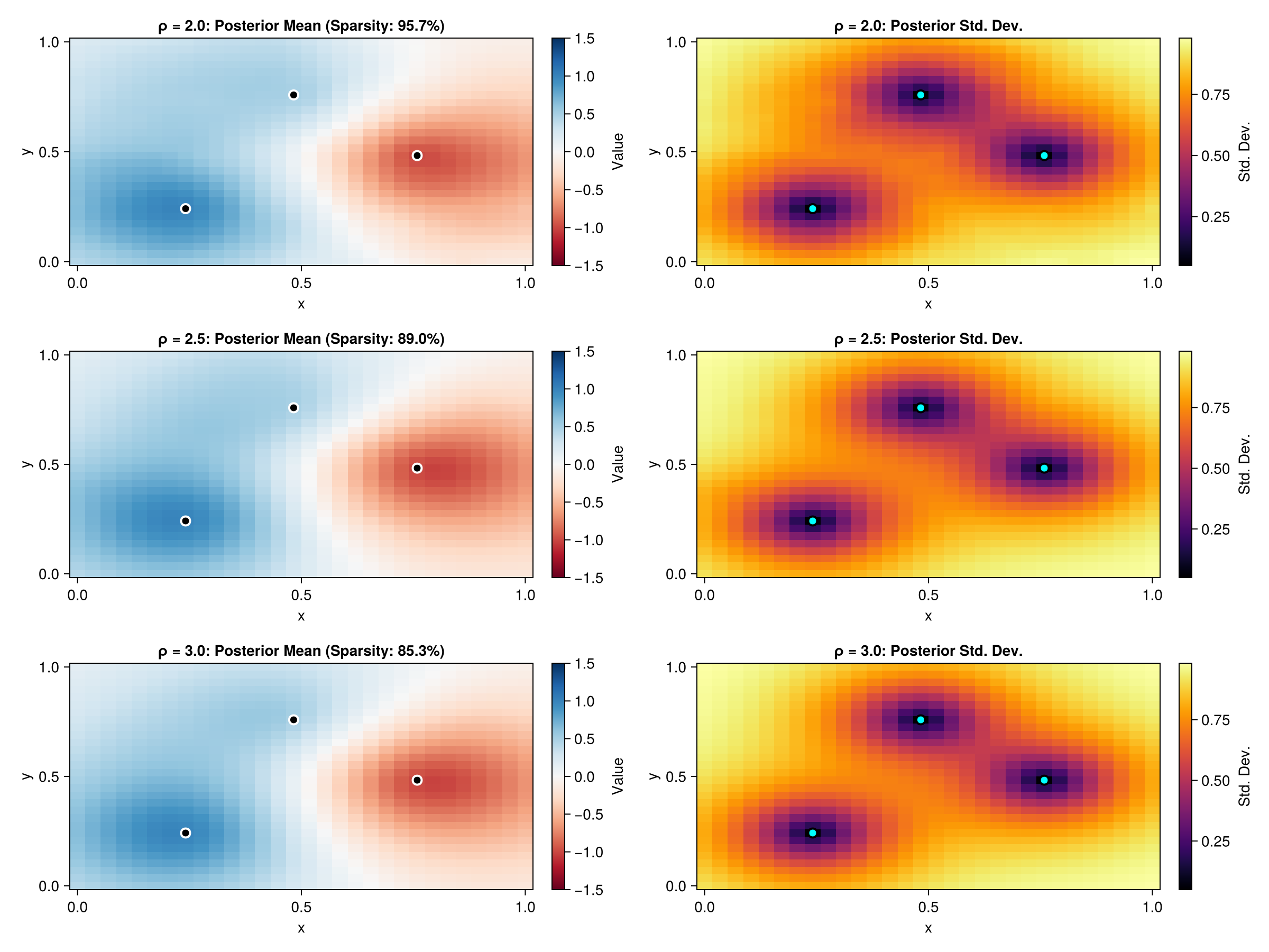

As ρ increases, the approximation becomes "crisper" and more accurate, better capturing the true Matern spatial correlation. However, this comes at the cost of reduced sparsity. The choice of ρ depends on the desired accuracy-efficiency tradeoff for your application.

Computational benefits

The main advantage of the sparse GMRF approximation is computational efficiency. Let's compare the memory footprint:

dense_memory = sizeof(K) / 1024^2  # MB
Q_posterior = precision_matrix(posterior)
sparse_memory = (sizeof(Q_posterior.rowval) + sizeof(Q_posterior.nzval) + sizeof(Q_posterior.colptr)) / 1024^2  # MB

println("\nMemory comparison:")
println("  Dense covariance matrix: $(round(dense_memory, digits = 2)) MB")
println("  Sparse precision matrix: $(round(sparse_memory, digits = 2)) MB")
println("  Memory reduction: $(round(100 * (1 - sparse_memory / dense_memory), digits = 1))%")

Memory comparison:
  Dense covariance matrix: 6.18 MB
  Sparse precision matrix: 0.54 MB
  Memory reduction: 91.2%

The computational footprint boils down to a dense Cholesky versus a sparse Cholesky. For fairly sparse matrices, a sparse Cholesky is often orders of magnitude faster than a dense Cholesky.

Thus, for larger problems (10,000+ points), the sparse representation enables computations that would be infeasible with the dense covariance matrix.

Comparison to the SPDE approach

The SPDE approach also produces a GMRF approximation of a Matern field. So which method is better?

The SPDE approach does not need the intermediate step of producing a covariance matrix. Thus I would expect it to be more efficient for the case of approximating evaluations of a Matern GP. However, the KL Cholesky approach is more flexible and generalizes easily to settings where we do not only care about point evaluations.

Conclusion

In this tutorial, we demonstrated how to use approximate_gmrf_kl to create sparse GMRF approximations from kernel matrices. This approach is extremely powerful due to its flexibility and its tendency to create very good approximations at relatively cheap cost.

The rho parameter controls the accuracy-sparsity tradeoff: larger values give more accurate approximations at the cost of reduced sparsity. For most applications, rho in the range [1.5, 3.0] provides a good balance.

For further details, we recommend reading [3] and checking the reference page KL-minimizing Sparse GP Approximations.

---

This page was generated using Literate.jl.