Spatiotemporal Modelling with SPDEs

In this tutorial, we will demonstrate how to perform spatiotemporal Bayesian inference using GMRFs based on a simple toy example.

Problem setup

Our goal is to model how a pollutant (i.e. some chemical) spreads across a river over time. We get (noisy) measurements of the pollutant concentration across the domain at time t = 0, and an additional measurement at some later point in time. To simplify things, we model the river as a 1D domain. Let's set up the problem:

x_left, x_right = -1.0, 1.0
Nₓ = 201
t_start, t_stop = 0.0, 1.0
Nₜ = 101
ts = range(t_start, t_stop, length = Nₜ)
f_initial = x -> exp(-(x + 0.6)^2 / 0.2^2)
xs_initial = range(x_left, x_right, length = Nₓ ÷ 2)
ys_initial = f_initial.(xs_initial)
noise_precision_initial = 0.1^(-2)

x_later = -0.25
y_later = 0.55
noise_precision_later = 0.01^(-2)

xs_all = [xs_initial; x_later]
ys_all = [ys_initial; y_later]
N_obs_all = length(ys_all)
101

Using GMRFs for spatiotemporal modelling

Fundamentally, we are interested in inferring a spatiotemporal function that models the pollutant concentration over time, which is an infinite-dimensional object. GMRFs, however, are finite-dimensional. This is not a limitation, it just means that we need to discretize space and time to ultimately obtain a discrete approximation to the infinite-dimensional object.

We're going to do this as follows:

  1. Set up a stochastic PDE (SPDE) that models the spatiotemporal, infinite-dimensional prior (a Gaussian process).
  2. Discretize the SPDE in space and time to obtain a GMRF which approximates the Gaussian process.
  3. Condition the GMRF on the observations to obtain the posterior.

Let's start by setting up our discretizations:

using GaussianMarkovRandomFields
using Ferrite

grid = generate_grid(Line, (Nₓ - 1,), Tensors.Vec(x_left), Tensors.Vec(x_right))
interpolation = Lagrange{RefLine,1}()
quadrature_rule = QuadratureRule{RefLine}(2)
disc = FEMDiscretization(grid, interpolation, quadrature_rule)
FEMDiscretization
  grid: Grid{1, Line, Float64} with 200 Line cells and 201 nodes
  interpolation: Lagrange{RefLine, 1}()
  quadrature_rule: QuadratureRule{RefLine, Vector{Float64}, Vector{Vec{1, Float64}}}
  # constraints: 0

A separable model

Perhaps the simplest spatiotemporal model is a separable one, where the spatial and temporal components are independent. We can model both the spatial and temporal components using Matern processes:

spde_space = MaternSPDE{1}(range = 0.2, smoothness = 1, σ² = 0.3)
spde_time = MaternSPDE{1}(range = 0.5, smoothness = 1)
MaternSPDE{1}(6.928203230275509, 3//2, 1.0, LinearAlgebra.UniformScaling{Bool}(true))

Discretize:

x_space = discretize(spde_space, disc)
Q_s = precision_map(x_space)

grid_time = generate_grid(Line, (Nₜ - 1,), Tensors.Vec(t_start), Tensors.Vec(t_stop))
disc_time = FEMDiscretization(grid_time, interpolation, quadrature_rule)
x_time = discretize(spde_time, disc_time)
Q_t = precision_map(x_time)
101×101 LinearMapWithSqrt{Float64}

Create the separable spatiotemporal model:

x_st_kron = kronecker_product_spatiotemporal_model(Q_t, Q_s, disc)
ConcreteConstantMeshSTGMRF{1, Float64}(
mean: [0.0, 0.0, 0.0, 0.0, 0.0, 0.0, 0.0, 0.0, 0.0, 0.0  …  0.0, 0.0, 0.0, 0.0, 0.0, 0.0, 0.0, 0.0, 0.0, 0.0]
precision: 20301×20301 LinearMapWithSqrt{Float64}
discretization: FEMDiscretization
  grid: Grid{1, Line, Float64} with 200 Line cells and 201 nodes
  interpolation: Lagrange{RefLine, 1}()
  quadrature_rule: QuadratureRule{RefLine, Vector{Float64}, Vector{Vec{1, Float64}}}
  # constraints: 0

solver_ref: Base.RefValue{AbstractSolver}(CholeskySolver{RBMCStrategy}([0.0, 0.0, 0.0, 0.0, 0.0, 0.0, 0.0, 0.0, 0.0, 0.0  …  0.0, 0.0, 0.0, 0.0, 0.0, 0.0, 0.0, 0.0, 0.0, 0.0], 20301×20301 LinearMapWithSqrt{Float64}, SparseArrays.CHOLMOD.Factor{Float64, Int64}
type:    LLt
method:  supernodal
maxnnz:  0
nnz:     2309004
success: true
, RBMCStrategy(100, Random.TaskLocalRNG()), nothing, nothing))
)

Great! Now let's condition on the observations. To do this, we construct a "spatial" observation matrix and transform it into a "spatiotemporal" observation matrix:

A_initial = evaluation_matrix(disc, [Tensors.Vec(x) for x in xs_initial])
t_initial_idx = 1 # Observe at first time point
A_initial = spatial_to_spatiotemporal(A_initial, t_initial_idx, Nₜ)
A_later = evaluation_matrix(disc, [Tensors.Vec(x_later)])
t_later_idx = 2 * Nₜ ÷ 3
A_later = spatial_to_spatiotemporal(A_later, t_later_idx, Nₜ)

A_all = [A_initial; A_later]

using LinearAlgebra, SparseArrays
Q_noise = sparse(I, N_obs_all, N_obs_all) * noise_precision_initial
Q_noise[end, end] = noise_precision_later
10000.0

Condition on the observations:

x_st_kron_posterior = condition_on_observations(x_st_kron, A_all, Q_noise, ys_all)
LinearConditionalGMRF of size 20301 and solver LinearConditionalCholeskySolver{RBMCStrategy}

Let's look at the dynamics of this posterior.

using CairoMakie
CairoMakie.activate!()
plot(x_st_kron_posterior, t_initial_idx)
Example block output
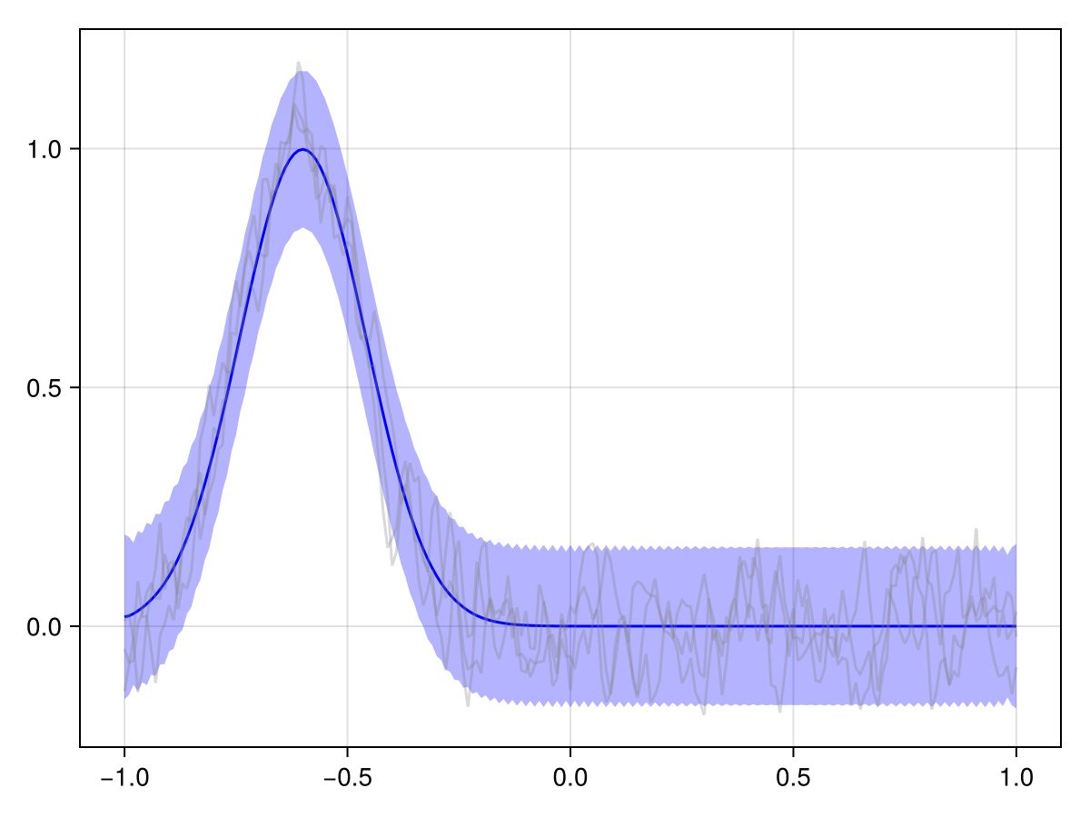
plot(x_st_kron_posterior, Nₜ ÷ 3)
Example block output
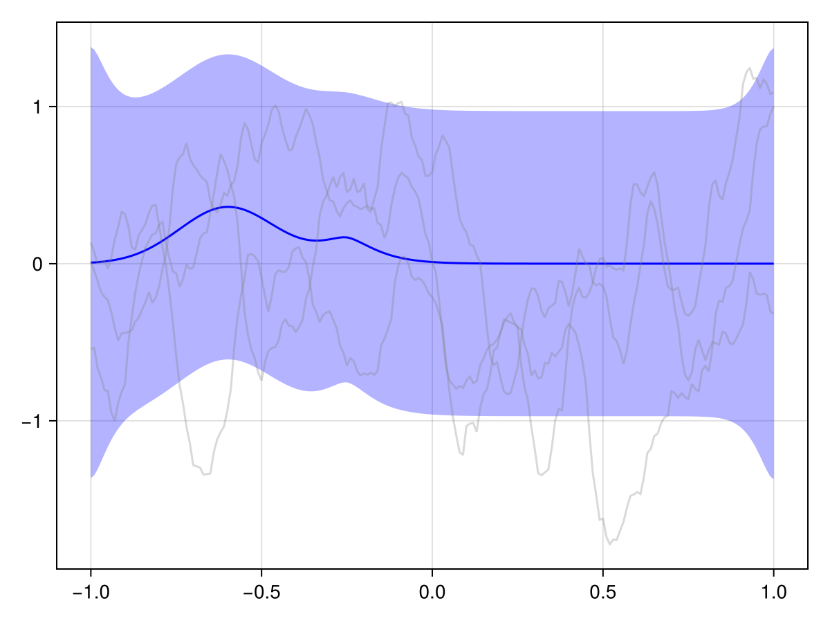
plot(x_st_kron_posterior, 2 * Nₜ ÷ 3)
Example block output
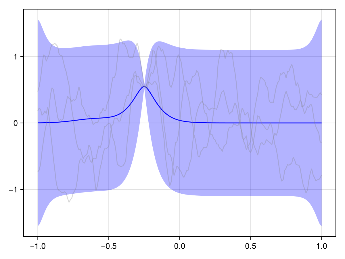
plot(x_st_kron_posterior, Nₜ)
Example block output

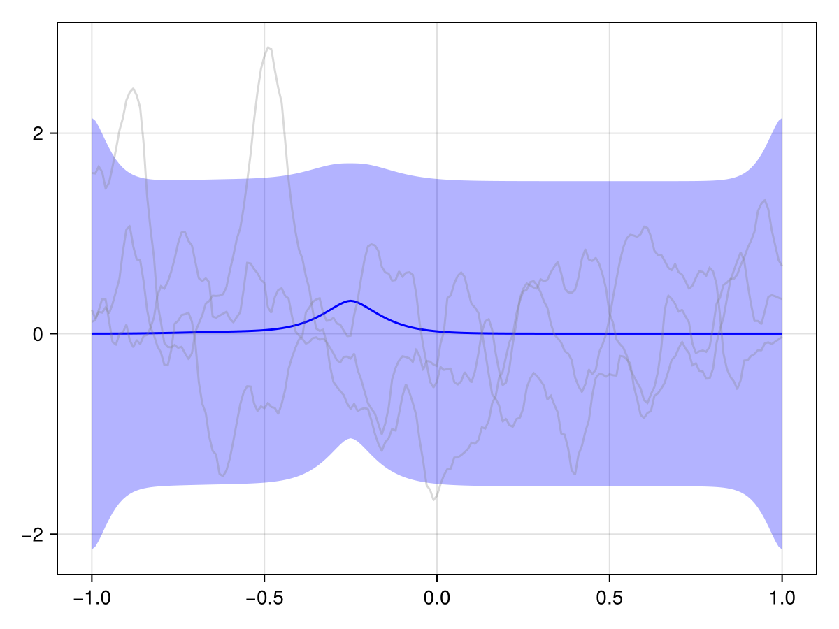
We see that the effect of our observations effectively just "dies off" over time. And generally in spatiotemporal statistics, this is a fair assumption: The further away in time we are from an observation, the less it should influence our predictions.

But in our case, we know a bit more about the phenomenon at hand. This is a river, and we know that it flows in a certain direction, and we probably also roughly know the flow speed. We should embed this information into our prior to get a more useful posterior!

Advection-diffusion priors

We can achieve this through a non-separable model that encodes these dynamics. Concretely, we are going to consider an advection-diffusion SPDE as presented in [2].

adv_diff_spde = AdvectionDiffusionSPDE{1}(
    γ = [-0.6],
    H = 0.1 * sparse(I, (1, 1)),
    τ = 0.1,
    α = 2 // 1,
    spatial_spde = spde_space,
    initial_spde = spde_space,
)
AdvectionDiffusionSPDE{1}(1.0, 2//1, sparse([1], [1], [0.1], 1, 1), [-0.6], 1.0, 0.1, MaternSPDE{1}(17.32050807568877, 3//2, 0.3, LinearAlgebra.UniformScaling{Bool}(true)), MaternSPDE{1}(17.32050807568877, 3//2, 0.3, LinearAlgebra.UniformScaling{Bool}(true)))

To discretize this SPDE, we only need a FEM discretization of space. For time, we simply specify the discrete time points which are then used internally for an implicit Euler scheme.

x_adv_diff = discretize(adv_diff_spde, disc, ts)
ImplicitEulerConstantMeshSTGMRF{1, Float64}(
mean: [0.0, 0.0, 0.0, 0.0, 0.0, 0.0, 0.0, 0.0, 0.0, 0.0  …  0.0, 0.0, 0.0, 0.0, 0.0, 0.0, 0.0, 0.0, 0.0, 0.0]
precision: 20301×20301 LinearMapWithSqrt{Float64}
discretization: FEMDiscretization
  grid: Grid{1, Line, Float64} with 200 Line cells and 201 nodes
  interpolation: Lagrange{RefLine, 1}()
  quadrature_rule: QuadratureRule{RefLine, Vector{Float64}, Vector{Vec{1, Float64}}}
  # constraints: 0

ssm: ImplicitEulerSSM(GMRF{Float64}(
mean: [0.0, 0.0, 0.0, 0.0, 0.0, 0.0, 0.0, 0.0, 0.0, 0.0  …  0.0, 0.0, 0.0, 0.0, 0.0, 0.0, 0.0, 0.0, 0.0, 0.0]
precision: 201×201 LinearMapWithSqrt{Float64}
solver_ref: Base.RefValue{AbstractSolver}(CholeskySolver{TakahashiStrategy}([0.0, 0.0, 0.0, 0.0, 0.0, 0.0, 0.0, 0.0, 0.0, 0.0  …  0.0, 0.0, 0.0, 0.0, 0.0, 0.0, 0.0, 0.0, 0.0, 0.0], 201×201 LinearMapWithSqrt{Float64}, SparseArrays.CHOLMOD.Factor{Float64, Int64}
type:    LLt
method:  simplicial
maxnnz:  600
nnz:     600
success: true
, TakahashiStrategy(), nothing, nothing))
)
, GaussianMarkovRandomFields.var"#104#109"{AdvectionDiffusionSPDE{1}}(AdvectionDiffusionSPDE{1}(1.0, 2//1, sparse([1], [1], [0.1], 1, 1), [-0.6], 1.0, 0.1, MaternSPDE{1}(17.32050807568877, 3//2, 0.3, LinearAlgebra.UniformScaling{Bool}(true)), MaternSPDE{1}(17.32050807568877, 3//2, 0.3, LinearAlgebra.UniformScaling{Bool}(true))), Core.Box(sparse([1, 2, 3, 1, 2, 3, 4, 1, 2, 3  …  199, 200, 201, 198, 199, 200, 201, 199, 200, 201], [1, 1, 1, 2, 2, 2, 2, 3, 3, 3  …  199, 199, 199, 200, 200, 200, 200, 201, 201, 201], [200.4000249999997, -300.4499999999995, 99.99999999999983, -299.84999999999945, 600.4000999999989, -400.4999999999993, 99.99999999999983, 99.99999999999983, -399.8999999999993, 600.4000999999989  …  600.4000999999989, -400.4999999999993, 99.99999999999983, 99.99999999999983, -399.8999999999993, 600.4000999999989, -300.4499999999995, 99.99999999999983, -299.84999999999945, 199.80002499999966], 201, 201)), Core.Box(sparse([1, 2, 1, 2, 3, 2, 3, 4, 3, 4  …  198, 199, 198, 199, 200, 199, 200, 201, 200, 201], [1, 1, 2, 2, 2, 3, 3, 3, 4, 4  …  198, 198, 199, 199, 199, 200, 200, 200, 201, 201], [0.005000000000000004, 0.0, 0.0, 0.010000000000000007, 0.0, 0.0, 0.010000000000000007, 0.0, 0.0, 0.010000000000000007  …  0.010000000000000007, 0.0, 0.0, 0.010000000000000007, 0.0, 0.0, 0.010000000000000007, 0.0, 0.0, 0.005000000000000004], 201, 201))), GaussianMarkovRandomFields.var"#107#112"(Core.Box(sparse([1, 2, 1, 2, 3, 2, 3, 4, 3, 4  …  198, 199, 198, 199, 200, 199, 200, 201, 200, 201], [1, 1, 2, 2, 2, 3, 3, 3, 4, 4  …  198, 198, 199, 199, 199, 200, 200, 200, 201, 201], [0.005000000000000004, 0.0, 0.0, 0.010000000000000007, 0.0, 0.0, 0.010000000000000007, 0.0, 0.0, 0.010000000000000007  …  0.010000000000000007, 0.0, 0.0, 0.010000000000000007, 0.0, 0.0, 0.010000000000000007, 0.0, 0.0, 0.005000000000000004], 201, 201))), GaussianMarkovRandomFields.var"#108#113"{SparseArrays.SparseMatrixCSC{Float64, Int64}}(sparse([1, 2, 3, 4, 5, 6, 7, 8, 9, 10  …  192, 193, 194, 195, 196, 197, 198, 199, 200, 201], [1, 2, 3, 4, 5, 6, 7, 8, 9, 10  …  192, 193, 194, 195, 196, 197, 198, 199, 200, 201], [199.99999999999986, 99.99999999999993, 99.99999999999993, 99.99999999999993, 99.99999999999993, 99.99999999999993, 100.00000000000047, 100.00000000000047, 99.99999999999993, 99.99999999999993  …  99.99999999999993, 99.99999999999993, 100.00000000000047, 100.00000000000047, 99.99999999999993, 99.99999999999993, 99.99999999999993, 99.99999999999993, 99.99999999999993, 199.99999999999986], 201, 201)), GaussianMarkovRandomFields.var"#105#110"{SparseArrays.SparseMatrixCSC{Float64, Int64}}(sparse([1, 2, 3, 4, 5, 6, 7, 8, 9, 10  …  192, 193, 194, 195, 196, 197, 198, 199, 200, 201], [1, 2, 3, 4, 5, 6, 7, 8, 9, 10  …  192, 193, 194, 195, 196, 197, 198, 199, 200, 201], [0.1, 0.1, 0.1, 0.1, 0.1, 0.1, 0.1, 0.1, 0.1, 0.1  …  0.1, 0.1, 0.1, 0.1, 0.1, 0.1, 0.1, 0.1, 0.1, 0.1], 201, 201)), GaussianMarkovRandomFields.var"#106#111"{SparseArrays.SparseMatrixCSC{Float64, Int64}}(sparse([1, 2, 3, 4, 5, 6, 7, 8, 9, 10  …  192, 193, 194, 195, 196, 197, 198, 199, 200, 201], [1, 2, 3, 4, 5, 6, 7, 8, 9, 10  …  192, 193, 194, 195, 196, 197, 198, 199, 200, 201], [10.0, 10.0, 10.0, 10.0, 10.0, 10.0, 10.0, 10.0, 10.0, 10.0  …  10.0, 10.0, 10.0, 10.0, 10.0, 10.0, 10.0, 10.0, 10.0, 10.0], 201, 201)), GMRF{Float64}(
mean: [0.0, 0.0, 0.0, 0.0, 0.0, 0.0, 0.0, 0.0, 0.0, 0.0  …  0.0, 0.0, 0.0, 0.0, 0.0, 0.0, 0.0, 0.0, 0.0, 0.0]
precision: 201×201 LinearMapWithSqrt{Float64}
solver_ref: Base.RefValue{AbstractSolver}(CholeskySolver{TakahashiStrategy}([0.0, 0.0, 0.0, 0.0, 0.0, 0.0, 0.0, 0.0, 0.0, 0.0  …  0.0, 0.0, 0.0, 0.0, 0.0, 0.0, 0.0, 0.0, 0.0, 0.0], 201×201 LinearMapWithSqrt{Float64}, SparseArrays.CHOLMOD.Factor{Float64, Int64}
type:    LLt
method:  simplicial
maxnnz:  600
nnz:     600
success: true
, TakahashiStrategy(), nothing, nothing))
)
, 0.0:0.01:1.0, ConstraintHandler{DofHandler{1, Grid{1, Line, Float64}}, Float64}(Dirichlet[], Int64[], [1, 2, 3, 4, 5, 6, 7, 8, 9, 10  …  192, 193, 194, 195, 196, 197, 198, 199, 200, 201], Float64[], Union{Nothing, Float64}[], Union{Nothing, Vector{Pair{Int64, Float64}}}[], Dict{Int64, Int64}(), Ferrite.BCValues{Float64}[], DofHandler{1, Grid{1, Line, Float64}}(SubDofHandler{DofHandler{1, Grid{1, Line, Float64}}}[SubDofHandler{DofHandler{1, Grid{1, Line, Float64}}}(DofHandler{1, Grid{1, Line, Float64}}(#= circular reference @-3 =#), OrderedCollections.OrderedSet{Int64}([1, 2, 3, 4, 5, 6, 7, 8, 9, 10  …  191, 192, 193, 194, 195, 196, 197, 198, 199, 200]), [:u], Interpolation[Lagrange{RefLine, 1}()], Int64[], 2)], [:u], [1, 2, 2, 3, 3, 4, 4, 5, 5, 6  …  196, 197, 197, 198, 198, 199, 199, 200, 200, 201], [1, 3, 5, 7, 9, 11, 13, 15, 17, 19  …  381, 383, 385, 387, 389, 391, 393, 395, 397, 399], [1, 1, 1, 1, 1, 1, 1, 1, 1, 1  …  1, 1, 1, 1, 1, 1, 1, 1, 1, 1], true, Grid{1, Line, Float64}(Line[Line((1, 2)), Line((2, 3)), Line((3, 4)), Line((4, 5)), Line((5, 6)), Line((6, 7)), Line((7, 8)), Line((8, 9)), Line((9, 10)), Line((10, 11))  …  Line((191, 192)), Line((192, 193)), Line((193, 194)), Line((194, 195)), Line((195, 196)), Line((196, 197)), Line((197, 198)), Line((198, 199)), Line((199, 200)), Line((200, 201))], Node{1, Float64}[Node{1, Float64}([-1.0]), Node{1, Float64}([-0.99]), Node{1, Float64}([-0.98]), Node{1, Float64}([-0.97]), Node{1, Float64}([-0.96]), Node{1, Float64}([-0.95]), Node{1, Float64}([-0.94]), Node{1, Float64}([-0.93]), Node{1, Float64}([-0.92]), Node{1, Float64}([-0.91])  …  Node{1, Float64}([0.91]), Node{1, Float64}([0.92]), Node{1, Float64}([0.93]), Node{1, Float64}([0.94]), Node{1, Float64}([0.95]), Node{1, Float64}([0.96]), Node{1, Float64}([0.97]), Node{1, Float64}([0.98]), Node{1, Float64}([0.99]), Node{1, Float64}([1.0])], Dict{String, OrderedCollections.OrderedSet{Int64}}(), Dict{String, OrderedCollections.OrderedSet{Int64}}(), Dict{String, OrderedCollections.OrderedSet{FacetIndex}}("left" => OrderedCollections.OrderedSet{FacetIndex}([FacetIndex((1, 1))]), "right" => OrderedCollections.OrderedSet{FacetIndex}([FacetIndex((200, 2))])), Dict{String, OrderedCollections.OrderedSet{VertexIndex}}()), 201), true), Float64[])
solver_ref: Base.RefValue{AbstractSolver}(CholeskySolver{RBMCStrategy}([0.0, 0.0, 0.0, 0.0, 0.0, 0.0, 0.0, 0.0, 0.0, 0.0  …  0.0, 0.0, 0.0, 0.0, 0.0, 0.0, 0.0, 0.0, 0.0, 0.0], 20301×20301 LinearMapWithSqrt{Float64}, SparseArrays.CHOLMOD.Factor{Float64, Int64}
type:    LLt
method:  supernodal
maxnnz:  0
nnz:     2727411
success: true
, RBMCStrategy(100, Random.TaskLocalRNG()), nothing, nothing))
)

Condition on the initial observations:

x_adv_diff_posterior = condition_on_observations(x_adv_diff, A_all, Q_noise, ys_all)
LinearConditionalGMRF of size 20301 and solver LinearConditionalCholeskySolver{RBMCStrategy}

Let's look at the dynamics of this posterior.

plot(x_adv_diff_posterior, t_initial_idx)
Example block output
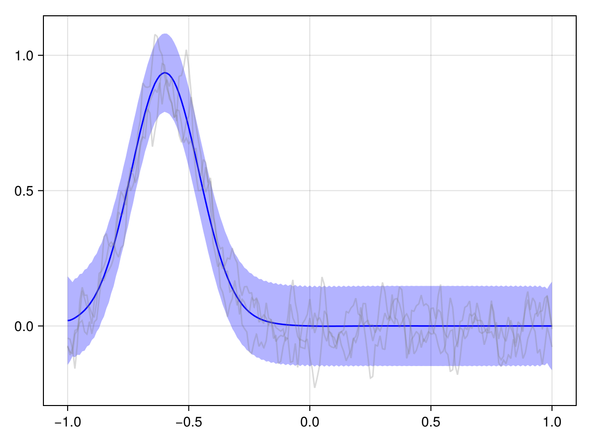
plot(x_adv_diff_posterior, Nₜ ÷ 3)
Example block output
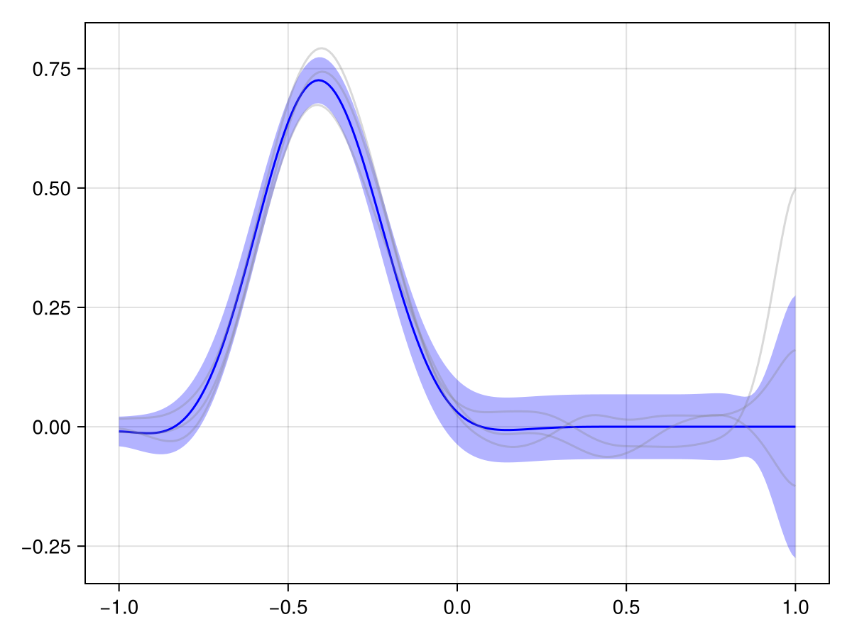
plot(x_adv_diff_posterior, 2 * Nₜ ÷ 3)
Example block output
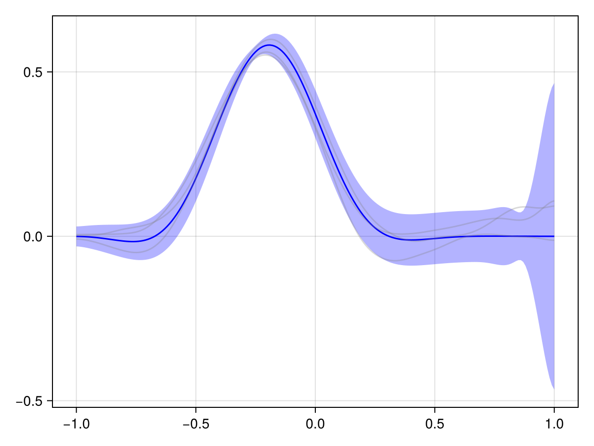
plot(x_adv_diff_posterior, Nₜ)
Example block output

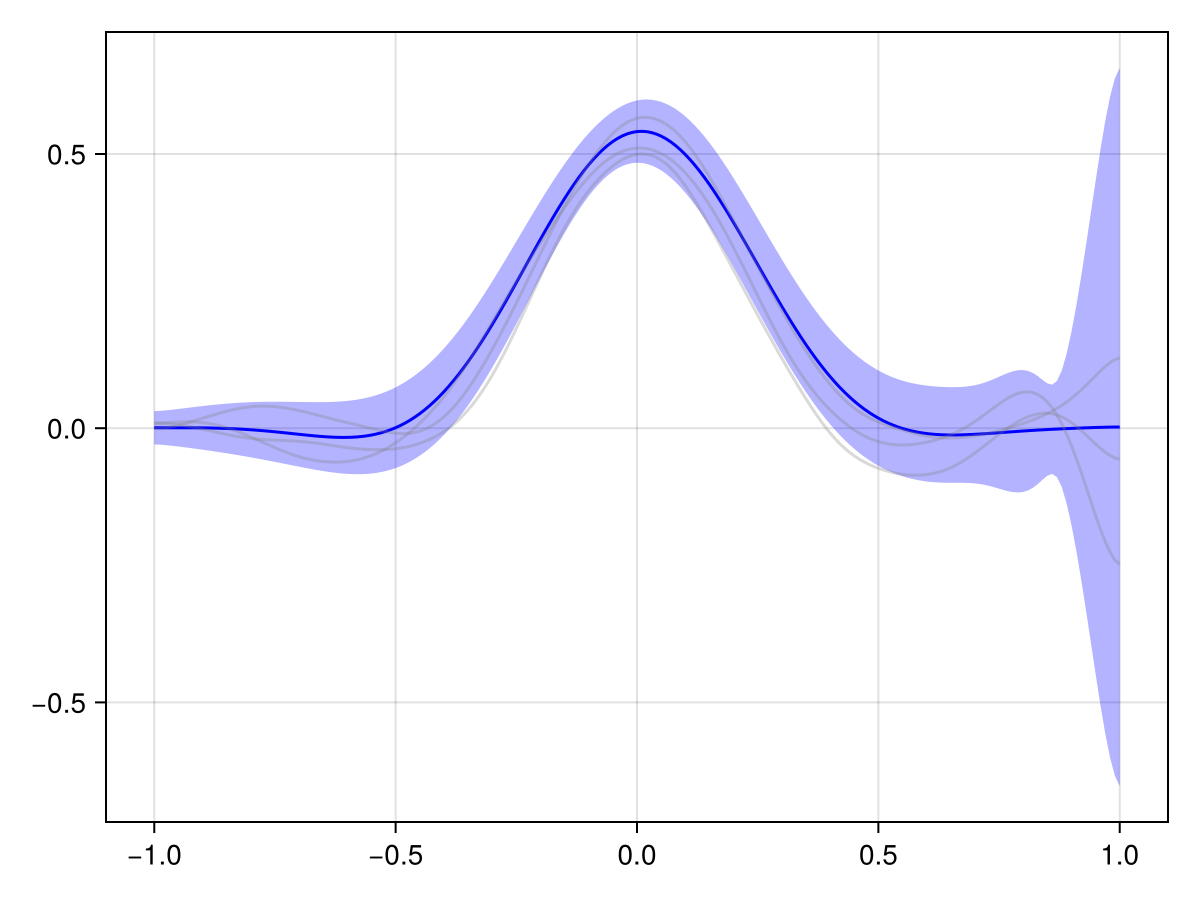
This looks much more reasonable! We see that the pollutant is transported downstream over time, and the observations at the later time point are consistent with this.

Conclusion

We have seen how to model spatiotemporal phenomena using GMRFs. We started with a simple separable model and then moved on to a more complex advection-diffusion model. The latter model was able to capture the dynamics of the river and the pollutant transport much better.

As mentioned initially, this was a simple toy example. But the underlying principles are the same for more complex problems. In particular, all of the above should work the same for arbitrary spatial meshes, as demonstrated e.g. in the tutorial Spatial Modelling with SPDEs.


This page was generated using Literate.jl.