Building autoregressive models

Introduction

In the following, we will construct a first-order auto-regressive model with Gaussian errors. Mathematically, this is expressed by

$$\begin{gathered} x_0\sim \mathcal{N}({\mu }_0,{\mathrm{\Lambda }}_0), \\ {x}_{t+1}=\varphi x_t+{\epsilon }_t,\epsilon \sim \mathcal{N}(0,\mathrm{\Lambda }). \end{gathered}$$

The latter equation is equivalent to the likelihood

$$x_{t+1}\mid x_t\sim \mathcal{N}(\varphi x_t,\mathrm{\Lambda }).$$

Under this model, the joint distribution over $x_1,\dots ,x_N$ (where $N$ is the number of steps) is Gaussian:

$$\left(\begin{array}{c}{x}_0\\ x_1\\ x_2\\ ⋮\\ x_{N-1}\\ x_N\end{array}\right)\sim \mathcal{N}(\left(\begin{array}{c}{\mu }_0\\ \varphi {\mu }_0\\ {\varphi }^2{\mu }_0\\ ⋮\\ {\varphi }^{N-1}{\mu }_0\\ {\varphi }^N{\mu }_0\end{array}\right),{\left(\begin{array}{ccccccc}{\mathrm{\Lambda }}_0& -\varphi & & & & & \\ -\varphi & \mathrm{\Lambda }+{\varphi }^2& -\varphi & & & & \\ & & & & & & \\ & & \ddots & \ddots & \ddots & & \\ & & & & & & \\ & & & & -\varphi & \mathrm{\Lambda }+{\varphi }^2& -\varphi \\ & & & & & -\varphi & \mathrm{\Lambda }\end{array}\right)}^{-1}).$$

The first-order Markov structure of the model results in a tridiagonal precision matrix. Thus, if we work with this Gaussian distribution in precision form (also commonly called information form), we gain tremendous computational benefits. By contrast, the covariance matrix of this Gaussian is fully dense.

More generally, this package deals with any sparse precision matrix, not just tridiagonal ones. Such Gaussians with sparse precision matrices are called GMRFs (short for Gaussian Markov Random Fields).

In the following, we construct a GMRF for the above first-order autoregressive model first manually by computing the mean and precision, and then automatically by simply specifying the parameters of the model.

Building an AR(1) model

We begin by loading GaussianMarkovRandomFields and LinearAlgebra.

using GaussianMarkovRandomFields, LinearAlgebra

We define a discretization of the real interval $[0,1]$, and specify some example parameters for the AR(1) model:

xs = 0:0.01:1
N = length(xs)
ρ = 0.995
τ = 3.0e4

30000.0

Now we compute the mean and the precision matrix of the joint distribution. We explicitly declare the precision matrix as a symmetric tridiagonal matrix, which unlocks highly efficient linear algebra routines for the underlying computations.

using LinearSolve
μ = [ρ^(i - 1) for i in eachindex(xs)]
main_diag = τ * [[1.0]; repeat([1.0 + ρ^2], N - 2); [1.0]]
off_diag = τ * repeat([-ρ], N - 1)
Q = SymTridiagonal(main_diag, off_diag)
x = GMRF(μ, Q, LinearSolve.LDLtFactorization())

GMRF{Float64} with 101 variables
  Algorithm: LinearSolve.LDLtFactorization{Nothing}
  Mean: [1.0, 0.995, 0.990025, ..., 0.6118738784280477, 0.6088145090359075, 0.6057704364907279]
  Q_sqrt: not available

A GMRF is a multivariate Gaussian, and it's compatible with Distributions.jl. We can get its mean, marginal standard deviation, and draw samples as follows:

using Plots, Distributions
plot(xs, mean(x), ribbon = 1.96 * std(x), label = "Mean + std")
for i in 1:3
    plot!(xs, rand(x), fillalpha = 0.3, linestyle = :dash, label = "Sample")
end
plot!()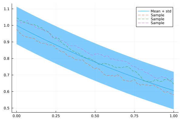

Great! Looks like an AR(1) model.

But what can you do with this? Well, for example you can use it as a prior for Bayesian inference. If we have a likelihood of the form

$$y\mid x\sim \mathcal{N}(Ax,{\mathrm{\Lambda }}_{\text{obs}}^{-1}),$$

then the posterior conditioned on these observations is again a GMRF, the moments of which we can compute in closed form.

In terms of code, the workflow for this is as follows:

1. Create a so-called "Observation Model". This basically defines the "category" of likelihood.

2. Instantiate a concrete likelihood from the model. This involves specifying concrete observations and hyperparameters.

3. Form a Gaussian approximation to the posterior under the prior and the observation likelihood.

In the case of linear Gaussian likelihoods, the "approximation" is of course exact, which our package leverages under the hood by dispatching to a closed-form expression.

import Distributions
obs_model = ExponentialFamily(Distributions.Normal, indices = [26, 76]) # Model
y = [0.85, 0.71]
obs_lik = obs_model(y; σ = 0.001) # Concrete likelihood
x_cond = gaussian_approximation(x, obs_lik)

GMRF{Float64} with 101 variables
  Algorithm: LinearSolve.LDLtFactorization{Nothing}
  Mean: [0.9716083556484854, 0.9664656840688296, 0.9613472955465625, ..., 0.6326547126518974, 0.6294914390886378, 0.6263439818931945]
  Q_sqrt: not available

Indeed, our model now conforms to these observations:

plot(xs, mean(x_cond), ribbon = 1.96 * std(x_cond), label = "Mean + std")
for i in 1:3
    plot!(xs, rand(x_cond), fillalpha = 0.3, linestyle = :dash, label = "Sample")
end
plot!()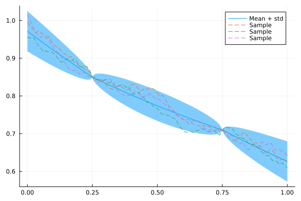

Latent models API

Above, we constructed the precision matrix of the AR1 GMRF manually. But of course, GaussianMarkovRandomFields.jl also provides utilities to construct common GMRF structures automatically. This is implemented through so-called "Latent Models".

The workflow is similar to that of Observation Models:

1. Construct a "Latent Model", which defines a "category" of GMRF structure.

2. Instantiate a concrete GMRF from the latent model. This involves specifying the concrete hyperparameter values.

latent_model = AR1Model(N)
x_ar1 = latent_model(ρ = ρ, τ = τ)

GMRF{Float64} with 101 variables
  Algorithm: LinearSolve.DefaultLinearSolver
  Mean: [0.0, 0.0, 0.0, ..., 0.0, 0.0, 0.0]
  Q_sqrt: not available

Beyond first-order models: CARs

You may have noticed that the AR(1) model above produces very rough samples. This may or may not be desirable, depending on the application. If we do want smoother samples, we can increase the order of the model. This adds off-diagonals to the precision matrix and thus reduces its sparsity, so computations become a bit more expensive. But it may be worth the overhead.

One model class to produce autoregressive models with flexible conditional dependencies and sparse precision matrices is that of conditional autoregressive models (_CAR_s). Such models are constructed based on a graph representation of the underlying data, where there is an edge between two nodes if they are conditionally dependent.

Let us construct an adjacency matrix that relates nodes not only to their immediate neighbors, but also to the neighbors' neighbors (a second-order model).

using SparseArrays
W = spzeros(N, N)
for i in 1:N
    for k in [-2, -1, 1, 2]
        j = i + k
        if 1 <= j <= N
            W[i, j] = 1.0
        end
    end
end

Now that we have the adjacency matrix, we can use a GaussianMarkovRandomFields.jl utility function to generate a CAR model from it, which internally constructs a slight variation of the graph Laplacian to form the precision matrix.

x_car = generate_car_model(W, 0.99; μ = μ, σ = 0.001)

GMRF{Float64} with 101 variables
  Algorithm: LinearSolve.DefaultLinearSolver
  Mean: [1.0, 0.995, 0.990025, ..., 0.6118738784280477, 0.6088145090359075, 0.6057704364907279]
  Q_sqrt: not available

Let's take our CAR for a test drive:

plot(xs, mean(x_car), ribbon = 1.96 * std(x_car), label = "Mean + std")
for i in 1:3
    plot!(xs, rand(x_car), fillalpha = 0.3, linestyle = :dash, label = "Sample")
end
plot!()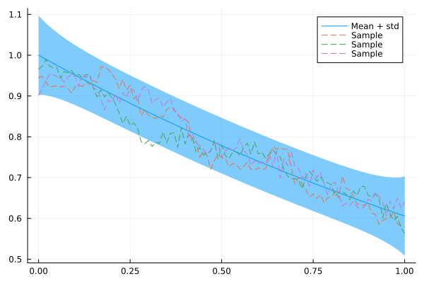

Let's see how this model fits data. We take the same observations as for the AR(1) model, but also add an observation for the starting point to reduce the uncertainty there.

obs_model = ExponentialFamily(Distributions.Normal, indices = [1, 26, 76])
y = [1.0, 0.85, 0.71]
obs_lik = obs_model(y; σ = 0.001)
x_car_cond = gaussian_approximation(x_car, obs_lik)
plot(xs, mean(x_car_cond), ribbon = 1.96 * std(x_car_cond), label = "Mean + std")
for i in 1:3
    plot!(xs, rand(x_car_cond), fillalpha = 0.3, linestyle = :dash, label = "Sample")
end
plot!()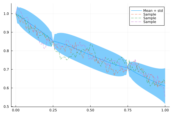

As expected, the interpolation of this model is less abrupt and spiky than for the AR(1) model.

Outlook

CAR models are quite flexible. Particularly for spatial data however, it is more common to model continuously through a Gaussian process. Fortunately, it turns out that popular Gaussian processes can be approximated quite nicely through GMRFs, allowing us to do the modelling in terms of a GP and the computations in terms of a GMRF. To learn more about this approach, check the tutorial on Spatial Modelling with SPDEs.

---

This page was generated using Literate.jl.