Boundary Conditions for SPDEs

In previous tutorials, we saw that we can approximate stochastic processes with GMRFs by discretizing stochastic partial differential equations (SPDEs). Such discretizations always involve boundary conditions, which specify the behavior of the process at the boundary of the domain. In the context of the finite element method, the simplest boundary condition is a homogeneous von Neumann boundary condition, which specifies that the derivative of the process normal to the boundary is zero. This approach is also used in the seminal work by Lindgren et al. [1].

Yet, in practice, this behavior is often not desirable. To circumvent boundary effects, people often artificially inflate the domain by adding a buffer zone around the data.

But what if we know the behavior of the process at the boundary, and it's not "the normal derivative is zero"? Fortunately, GaussianMarkovRandomFields.jl interfaces rather smoothly with Ferrite.jl, which we can use to specify more complex boundary conditions. Let's see how this works.

Spatial example: Matern SPDE

We start by specifying a mesh over the interval [-1, 1].

using GaussianMarkovRandomFields, Ferrite
grid = generate_grid(Line, (50,))
interpolation = Lagrange{RefLine, 1}()
quadrature_rule = QuadratureRule{RefLine}(2)

QuadratureRule{RefLine, Vector{Float64}, Vector{Vec{1, Float64}}}([0.9999999999999998, 0.9999999999999998], Vec{1, Float64}[[-0.5773502691896257], [0.5773502691896257]])

Dirichlet boundary

Let us now use Ferrite to define a homogeneous Dirichlet boundary condition, which specifies that the process is zero at the boundary.

function get_dirichlet_constraint(grid::Ferrite.Grid{1})
    boundary = getfacetset(grid, "left") ∪ getfacetset(grid, "right")

    return Dirichlet(:u, boundary, x -> (x[1] ≈ -1.0) ? 0.0 : (x[1] ≈ 1.0) ? 0.0 : 0.0)
end

dbc = get_dirichlet_constraint(grid)

Dirichlet(Main.var"#1#2"(), OrderedCollections.OrderedSet{FacetIndex}(FacetIndex[FacetIndex((1, 1)), FacetIndex((50, 2))]), :u, Int64[], Int64[], Int64[])

GaussianMarkovRandomFields.jl supports such boundary conditions in a "soft" way. This means that we enforce the boundary conditions up to noise of a certain, user-specified magnitude. This ensures that the resulting GMRF has full rank. If you don't care much for probabilistic boundary conditions, you can just set the noise to a sufficiently small value.

bcs = [(dbc, 1.0e-4)] # 1e-4 is the noise in terms of the standard deviation

1-element Vector{Tuple{Dirichlet, Float64}}:
 (Dirichlet(Main.var"#1#2"(), OrderedCollections.OrderedSet{FacetIndex}(FacetIndex[FacetIndex((1, 1)), FacetIndex((50, 2))]), :u, Int64[], Int64[], Int64[]), 0.0001)

We can now create a FEM discretization with the specified boundary conditions.

disc = FEMDiscretization(grid, interpolation, quadrature_rule, [(:u, nothing)], bcs)

FEMDiscretization
  grid: Grid{1, Line, Float64} with 50 Line cells and 51 nodes
  interpolation: Lagrange{RefLine, 1}()
  quadrature_rule: QuadratureRule{RefLine, Vector{Float64}, Vector{Vec{1, Float64}}}
  # constraints: 2

Let's now define some Matern SPDE and discretize it.

matern_spde = MaternSPDE{1}(range = 0.5, smoothness = 1, σ² = 0.3)
x = discretize(matern_spde, disc)

GMRF{Float64} with 51 variables
  Algorithm: LinearSolve.DefaultLinearSolver
  Mean: [0.0, 0.0, 0.0, ..., 0.0, 0.0, 0.0]
  Q_sqrt: available

Verify for yourself that the boundary value is zero for all samples, and that the variance vanishes at the boundary:

using CairoMakie
CairoMakie.activate!()
plot(x, disc)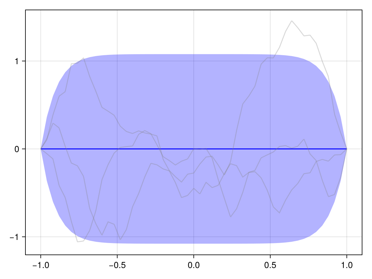

Periodic boundary

We can also define a periodic boundary condition in terms of an affine constraint:

function get_periodic_constraint(grid::Ferrite.Grid{1})
    cellidx_left, dofidx_left = collect(grid.facetsets["left"])[1]
    cellidx_right, dofidx_right = collect(grid.facetsets["right"])[1]

    temp_dh = DofHandler(grid)
    add!(temp_dh, :u, Lagrange{RefLine, 1}())
    close!(temp_dh)
    cc = CellCache(temp_dh)
    get_dof(cell_idx, dof_idx) = (reinit!(cc, cell_idx); celldofs(cc)[dof_idx])
    dof_left = get_dof(cellidx_left, dofidx_left)
    dof_right = get_dof(cellidx_right, dofidx_right)

    return AffineConstraint(dof_left, [dof_right => 1.0], 0.0)
end

pbc = get_periodic_constraint(grid)

AffineConstraint{Float64}(1, [51 => 1.0], 0.0)

The rest of the procedure is analogous to the Dirichlet case:

bcs = [(pbc, 1.0e-4)]
disc_periodic =
    FEMDiscretization(grid, interpolation, quadrature_rule, [(:u, nothing)], bcs)
x_periodic = discretize(matern_spde, disc_periodic)

GMRF{Float64} with 51 variables
  Algorithm: LinearSolve.DefaultLinearSolver
  Mean: [0.0, 0.0, 0.0, ..., 0.0, 0.0, 0.0]
  Q_sqrt: available

Verify for yourself that the values at the left and right boundary match for all samples:

plot(x_periodic, disc)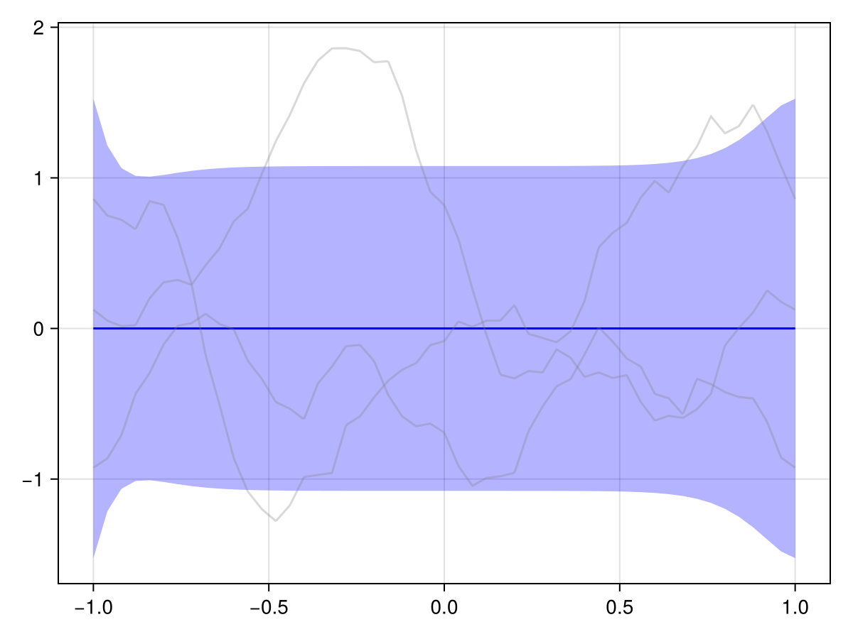

Spatiotemporal example: Advection-Diffusion SPDE

This works just as well in the spatiotemporal case. Let's reuse our previous discretization for a 1D advection-diffusion SPDE:

using LinearAlgebra, SparseArrays
spde = AdvectionDiffusionSPDE{1}(
    γ = [-0.6],
    H = 0.1 * sparse(I, (1, 1)),
    τ = 0.1,
    α = 2 // 1,
    spatial_spde = matern_spde,
    initial_spde = matern_spde,
)
ts = 0:0.05:1
N_t = length(ts)
x_adv_diff_dirichlet = discretize(spde, disc, ts)
x_adv_diff_periodic = discretize(spde, disc_periodic, ts)

MetaGMRF{ImplicitEulerMetadata}
  Inner GMRF: GMRF{Float64}(n=1071, alg=LinearSolve.DefaultLinearSolver)
  Metadata: ImplicitEulerMetadata{1}(51 spatial × 21 time)

To make things clearer, we are going to condition these GMRFs on a Gaussian initial condition to see how it propagates over time.

xs_ic = -0.99:0.01:0.99
ys_ic = exp.(-xs_ic .^ 2 / 0.2^2)
A_ic = evaluation_matrix(disc, [Tensors.Vec(x) for x in xs_ic])
A_ic = spatial_to_spatiotemporal(A_ic, 1, N_t)

x_adv_diff_dirichlet = condition_on_observations(x_adv_diff_dirichlet, A_ic, 1.0e8, ys_ic)
x_adv_diff_periodic = condition_on_observations(x_adv_diff_periodic, A_ic, 1.0e8, ys_ic)

MetaGMRF{ImplicitEulerMetadata}
  Inner GMRF: GMRF{Float64}(n=1071, alg=LinearSolve.DefaultLinearSolver)
  Metadata: ImplicitEulerMetadata{1}(51 spatial × 21 time)

First, check the initial observations:

plot(x_adv_diff_dirichlet, 1)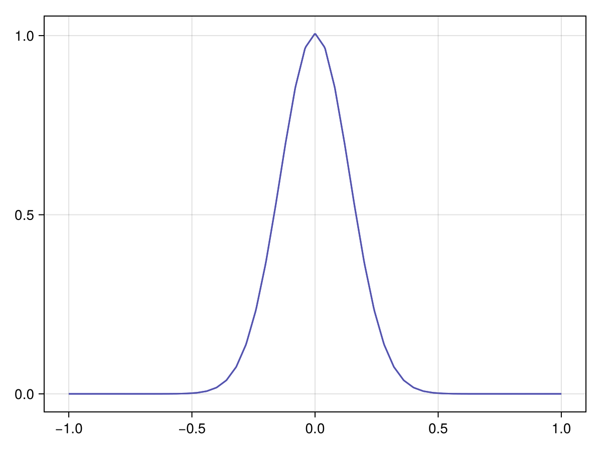

Now, let's see how the process evolves over time:

plot(x_adv_diff_dirichlet, N_t ÷ 2)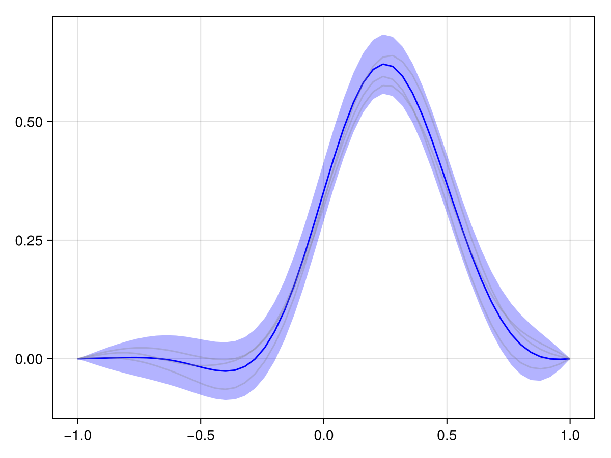

plot(x_adv_diff_dirichlet, N_t)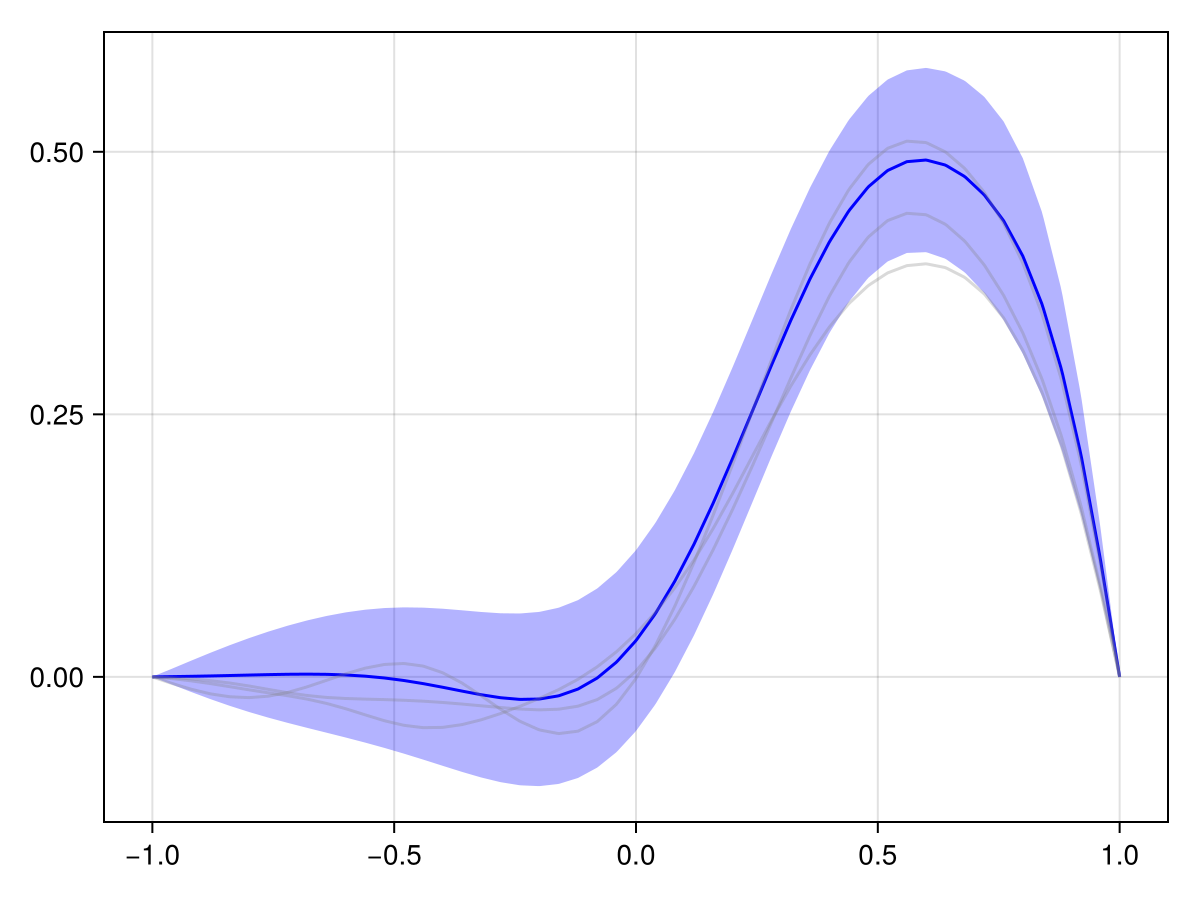

Compare to this to the periodic case:

plot(x_adv_diff_periodic, N_t ÷ 2)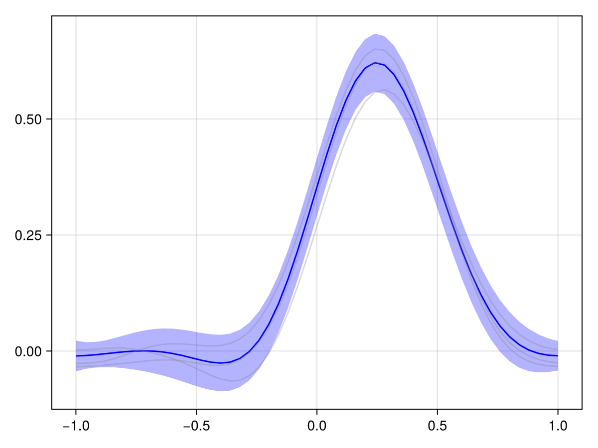

plot(x_adv_diff_periodic, N_t)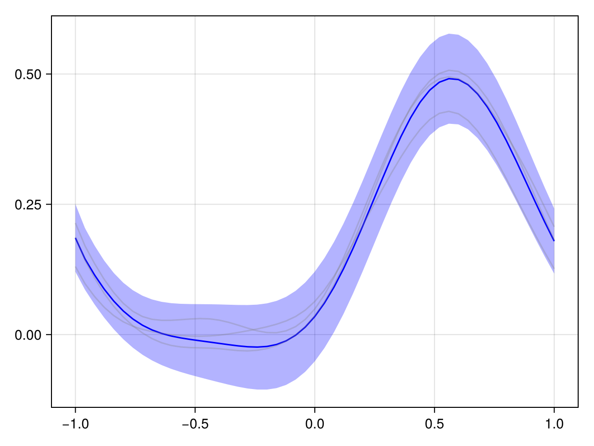

Conclusion

We have seen how to specify more complex boundary conditions for GMRFs. All it takes is to construct the boundary conditions in Ferrite and add some noise.

For the sake of simplicity, this tutorial considered discretizations of a one-dimensional interval, but of course the same principles apply to higher dimensions and more complex geometries.

---

This page was generated using Literate.jl.