Bernoulli Spatial Classification with a Matérn Field

In this walkthrough you will build a simple probabilistic classifier for spatial point data with binary labels. We combine:

a spatial latent Gaussian field with a Matérn covariance (via SPDE), and
a Bernoulli observation model with a logit link for classification.

You will learn how to:

construct a Matérn latent model from coordinates,
connect it to Bernoulli observations,
perform a fast Gaussian approximation to the posterior, and
make and visualize spatial probability predictions on a grid.

We use the well-known Lansing Woods dataset (tree locations with species marks). The dataset here provides three columns: x, y, is_hickory (0/1). We try a local file first so the tutorial works offline; otherwise we download a small RDA file from the upstream repository.

julia

using DataFrames
using GaussianMarkovRandomFields
using LinearAlgebra, Random
using Plots

Load data (local if present, otherwise download)

julia

using CodecBzip2, RData
data_dir = joinpath(@__DIR__, "data")
mkpath(data_dir)
local_rda = joinpath(data_dir, "lansing_trees.rda")

if !isfile(local_rda)
    repo_url = "https://github.com/spatstat/spatstat.data/raw/refs/heads/master/data/lansing.rda"
    try
        download(repo_url, local_rda)
    catch err
        error(
            "Could not download dataset (are you offline?). " *
                "Place an RData file at $(local_rda) or pass your own DataFrame."
        )
    end
end

objs = RData.load(local_rda)["lansing"]
x, y = objs[objs.name2index["x"]], objs[objs.name2index["y"]]
is_hickory = objs[objs.name2index["marks"]] .== "hickory"

df = DataFrame(["x" => x, "y" => y, "is_hickory" => is_hickory])
df = unique(df)  # remove any accidental duplicates
first(df, 5)     # show a preview in the docs

5×3 DataFrame

Row	x	y	is_hickory
	Float64	Float64	Bool
1	0.078	0.091	false
2	0.076	0.266	false
3	0.051	0.225	false
4	0.015	0.366	false
5	0.03	0.426	false

Coordinates and binary label (1=hickory, 0=other)

julia

X = Matrix(df[:, [:x, :y]])
y = Vector{Int}(df[:, :is_hickory])

2250-element Vector{Int64}:
 0
 0
 0
 0
 0
 0
 0
 0
 0
 0
 ⋮
 0
 0
 0
 0
 0
 0
 0
 0
 0

Train/test split

We take a random 80/20 split for a quick, reproducible evaluation.

julia

Random.seed!(42)
n = size(X, 1)
perm = randperm(n)
split = round(Int, 0.8n)
train_idcs = perm[1:split]
test_idcs = perm[(split + 1):end]

X_train, y_train = X[train_idcs, :], y[train_idcs]
X_test, y_test = X[test_idcs, :], y[test_idcs]

([0.497 0.562; 0.756 0.793; … ; 0.718 0.411; 0.17 0.085], [0, 0, 0, 0, 0, 0, 0, 0, 1, 1  …  1, 0, 1, 1, 0, 0, 0, 0, 0, 0])

Latent model: Matérn GP via SPDE

We construct a spatial latent model from the observation coordinates. Under the hood this builds a sparse SPDE representation of a Matérn Gaussian field.

Key hyperparameters:

smoothness: controls differentiability of the field. We use 1 by default which is a common choice for spatial classification.
range: controls the distance over which the field exhibits strong correlation. As a rule of thumb, set it to a fraction of the spatial extent of your data.

julia

latent = MaternModel(X; smoothness = 1)
u = latent(range = 0.2)  # tune this to your dataset's scale

GMRF{Float64} with 8321 variables
  Algorithm: LinearSolve.DefaultLinearSolver
  Mean: [0.0, 0.0, 0.0, ..., 0.0, 0.0, 0.0]
  Q_sqrt: not available

Bernoulli observations (logit link)

We connect the latent field to point-wise labels using a Bernoulli exponential family model with a logit link. The model is evaluated at the observed locations.

julia

import Distributions
obs_model = PointEvaluationObsModel(latent.discretization, X_train, Distributions.Bernoulli)
lik = obs_model(y_train)

LinearlyTransformedLikelihood{BernoulliLikelihood{LogitLink, Nothing}, SparseArrays.SparseMatrixCSC{Float64, Int64}}(BernoulliLikelihood{LogitLink, Nothing}(LogitLink(), [1, 0, 0, 1, 0, 1, 1, 1, 0, 0  …  0, 0, 1, 0, 0, 0, 1, 1, 0, 0], nothing), sparse([1150, 1737, 1737, 1737, 1544, 1544, 1544, 84, 84, 84  …  540, 416, 1777, 1198, 212, 1691, 1137, 1712, 1110, 884], [1, 4, 5, 6, 7, 8, 9, 10, 11, 12  …  8263, 8265, 8271, 8272, 8283, 8286, 8292, 8294, 8304, 8311], [3.774758283725532e-15, 1.0000000000000007, -1.4988010832439613e-15, 8.326672684688674e-16, -3.219646771412954e-15, -1.887379141862766e-15, 1.0000000000000049, 1.000000000000002, -2.220446049250313e-15, 2.220446049250313e-16  …  0.999999999999996, 1.0000000000000009, 0.9999999999999938, 1.0000000000000044, 1.0000000000000022, 1.000000000000002, 1.0000000000000175, 0.9999999999999927, 1.0000000000000069, 0.9999999999999942], 1800, 8321))

Inference: Gaussian approximation

We perform a Gaussian approximation of the posterior for the latent field u given the Bernoulli observations. This is typically very fast thanks to the sparse structure of the SPDE discretization.

julia

post = gaussian_approximation(u, lik)

GMRF{Float64} with 8321 variables
  Algorithm: LinearSolve.DefaultLinearSolver
  Mean: [0.3307662784795072, 0.04608798139458996, 0.01674607454557331, ..., 0.5858919864374935, 0.8286802714848384, -0.2802357564000051]
  Q_sqrt: not available

Evaluation on held-out data

To score the classifier we predict probabilities at test locations. The helper conditional_distribution returns the predictive distribution of the linear predictor at new points; taking mean applies the Bernoulli mean transform under the logit link to yield probabilities in [0,1].

julia

obs_model_test = PointEvaluationObsModel(latent.discretization, X_test, Distributions.Bernoulli)
pred_dist_test = conditional_distribution(obs_model_test, mean(post))

Distributions.Product{Distributions.Discrete, Distributions.Bernoulli{Float64}, Vector{Distributions.Bernoulli{Float64}}}(
v: Distributions.Bernoulli{Float64}[Distributions.Bernoulli{Float64}(p=0.21028351508236026), Distributions.Bernoulli{Float64}(p=0.2676284375255825), Distributions.Bernoulli{Float64}(p=0.38383476092144847), Distributions.Bernoulli{Float64}(p=0.2606682467389828), Distributions.Bernoulli{Float64}(p=0.2108838920589112), Distributions.Bernoulli{Float64}(p=0.36373811981485776), Distributions.Bernoulli{Float64}(p=0.585830457080814), Distributions.Bernoulli{Float64}(p=0.14389938593096208), Distributions.Bernoulli{Float64}(p=0.24316534500131815), Distributions.Bernoulli{Float64}(p=0.5448418293764192)  …  Distributions.Bernoulli{Float64}(p=0.4461312217757518), Distributions.Bernoulli{Float64}(p=0.1604720899451638), Distributions.Bernoulli{Float64}(p=0.6760532622845694), Distributions.Bernoulli{Float64}(p=0.29273390878077377), Distributions.Bernoulli{Float64}(p=0.20438189935179307), Distributions.Bernoulli{Float64}(p=0.06511783064651357), Distributions.Bernoulli{Float64}(p=0.31011933350280824), Distributions.Bernoulli{Float64}(p=0.26050723815563426), Distributions.Bernoulli{Float64}(p=0.40201966063552363), Distributions.Bernoulli{Float64}(p=0.11953872778116378)]
)

Convert to probabilities and class labels (0/1) using a 0.5 threshold.

julia

ŷ_prob = mean(pred_dist_test)  # probability for class "hickory"
ŷ = Int.(ŷ_prob .>= 0.5)

accuracy = sum(ŷ .== y_test) / length(y_test)
accuracy

0.74

Visualization

A simple heatmap of predicted probabilities with all observed points overlaid. Redder areas indicate higher probability of class "hickory".

julia

xmin, xmax = extrema(X[:, 1])
ymin, ymax = extrema(X[:, 2])
nx, ny = 100, 100
xs = range(xmin, xmax; length = nx)
ys = range(ymin, ymax; length = ny)

grid_points = Array{Float64}(undef, nx * ny, 2)
for (i, (yv, xv)) in enumerate(Iterators.product(ys, xs))
    grid_points[i, 1] = xv
    grid_points[i, 2] = yv
end

obs_grid = PointEvaluationObsModel(latent.discretization, grid_points, Distributions.Bernoulli)
pred_grid = conditional_distribution(obs_grid, mean(post))
probs = reshape(mean(pred_grid), (nx, ny))

plt = heatmap(
    xs, ys, probs; xlabel = "x", ylabel = "y",
    title = "P(is_hickory=1) — acc=$(round(accuracy, digits = 3))",
    colorbar = true, legend = :topright
)

class0 = findall(==(0), y)
class1 = findall(==(1), y)

scatter!(plt, X[class1, 1], X[class1, 2]; m = :circle, ms = 1.5, c = :tomato, label = "hickory")
scatter!(plt, X[class0, 1], X[class0, 2]; m = :circle, ms = 1.5, c = :royalblue, label = "other")
plt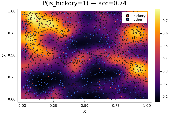

Notes and tips

Hyperparameters matter: start by adjusting range so the spatial field varies on a scale similar to your data. If predictions look too smooth or too noisy, increase or decrease range respectively.
Performance scales well: the SPDE discretization yields sparse matrices, making inference and prediction efficient for thousands to millions of points.
Your own data: if you already have a DataFrame with columns :x, :y, and a boolean/0-1 label column, set df accordingly and keep the rest unchanged.
Offline runs: if the download step fails, add your file at docs/src/literate-tutorials/data/lansing_trees.rda or point df to your data.

This page was generated using Literate.jl.

Bernoulli Spatial Classification with a Matérn Field ​

Load data (local if present, otherwise download) ​

Train/test split ​

Latent model: Matérn GP via SPDE ​

Bernoulli observations (logit link) ​

Inference: Gaussian approximation ​

Evaluation on held-out data ​

Visualization ​

Notes and tips ​

Bernoulli Spatial Classification with a Matérn Field

Load data (local if present, otherwise download)

Train/test split

Latent model: Matérn GP via SPDE

Bernoulli observations (logit link)

Inference: Gaussian approximation

Evaluation on held-out data

Visualization

Notes and tips