Spatial Modelling with SPDEs

Data preprocessing

In the following, we are going to work with the meuse dataset. This dataset contains measurements of zinc concentrations in the soil near the Meuse river.

We begin by downloading the dataset.

meuse_path = joinpath(@__DIR__, "meuse.csv")
meuse_URL = "https://gist.githubusercontent.com/essicolo/91a2666f7c5972a91bca763daecdc5ff/raw/056bda04114d55b793469b2ab0097ec01a6d66c6/meuse.csv"
download(meuse_URL, meuse_path)

"/home/runner/work/GaussianMarkovRandomFields.jl/GaussianMarkovRandomFields.jl/docs/build/tutorials/meuse.csv"

We load the CSV file into a DataFrame and inspect the first few rows.

using CSV, DataFrames
df = DataFrame(CSV.File(meuse_path))
df[1:5, [:x, :y, :zinc]]

Let us visualize the data. We plot the zinc concentrations as a function of the x and y coordinates.

using Plots
x = convert(Vector{Float64}, df[:, :x])
y = convert(Vector{Float64}, df[:, :y])
zinc = df[:, :zinc]
scatter(x, y, zcolor = zinc)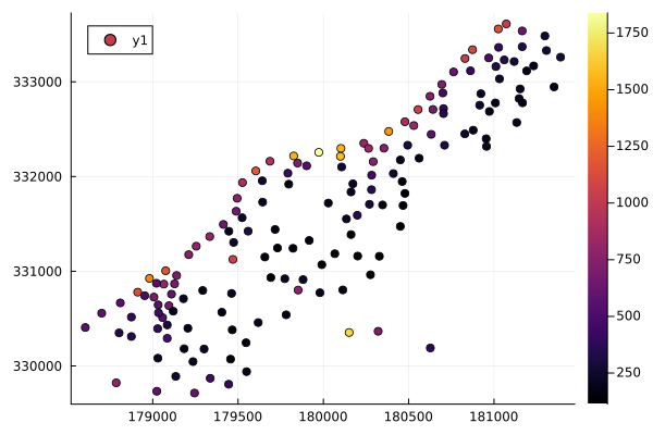

Finally, in classic machine learning fashion, we split the data into a training and a test set. We use about 85% of the data for training and the remaining 15% for testing.

using Random
train_idcs = randsubseq(1:size(df, 1), 0.85)
test_idcs = [i for i = 1:size(df, 1) if isempty(searchsorted(train_idcs, i))]
X = [x y]
X_train = X[train_idcs, :]
X_test = X[test_idcs, :]
y_train = zinc[train_idcs]
y_test = zinc[test_idcs]
size(X_train, 1), size(X_test, 1)

(135, 20)

Spatial Modelling

Matern Gaussian processes (GPs) are a powerful model class commonly used in geostatistics for such data. Unfortunately, without using any further tricks, GPs have a cubic runtime complexity. As the size of the dataset grows, this quickly becomes prohibitively expensive. In the tutorial on Autoregressive models, we learned that GMRFs enable highly efficient Gaussian inference through sparse precision matrices. Can we combine the modelling power of GPs with the efficiency of GMRFs?

Yes, we can: [1] told us how. It turns out that Matern processes may equivalently be interpreted as solutions of certain stochastic partial differential equations (SPDEs). If we discretize this SPDE appropriately – for example using the finite element method (FEM) – we get a discrete GMRF approximation of a Matern process. The approximation quality improves as the resolution of the FEM mesh increases. If this all sounds overly complicated to you, fear not! GaussianMarkovRandomFields.jl takes care of the technical details for you, so you can focus on the modelling.

We start by generating a FEM mesh for our data. Internally, GaussianMarkovRandomFields.jl computes a convex hull around the scattered data and then extends it slightly to counteract effects from the boundary condition of the SPDE.

The final output is a Ferrite.jl grid. We can also save the generated mesh, e.g. to visualize it via Gmsh.

using GaussianMarkovRandomFields
points = zip(x, y)
grid = generate_mesh(points, 600.0, 100.0, save_path = "meuse.msh")

Grid{2, Triangle, Float64} with 2143 Triangle cells and 1119 nodes

We can now create a FEM discretization, which consists of the grid, a choice of basis functions, and a quadrature rule.

using Ferrite
ip = Lagrange{RefTriangle,1}()
qr = QuadratureRule{RefTriangle}(2)
disc = FEMDiscretization(grid, ip, qr)

FEMDiscretization
  grid: Grid{2, Triangle, Float64} with 2143 Triangle cells and 1119 nodes
  interpolation: Lagrange{RefTriangle, 1}()
  quadrature_rule: QuadratureRule{RefTriangle, Vector{Float64}, Vector{Vec{2, Float64}}}
  # constraints: 0

We now create a Matern SPDE and discretize it. While we could specify the Matern SPDE in terms of its direct parameters κ and ν, we here choose to specify it through the more easily interpretable parameters range and smoothness.

spde = MaternSPDE{2}(range = 400.0, smoothness = 1)
u_matern = discretize(spde, disc)

GMRF{Float64}(
mean: [0.0, 0.0, 0.0, 0.0, 0.0, 0.0, 0.0, 0.0, 0.0, 0.0  …  0.0, 0.0, 0.0, 0.0, 0.0, 0.0, 0.0, 0.0, 0.0, 0.0]
precision: 1119×1119 LinearMapWithSqrt{Float64}
solver_ref: Base.RefValue{AbstractSolver}(CholeskySolver{TakahashiStrategy}([0.0, 0.0, 0.0, 0.0, 0.0, 0.0, 0.0, 0.0, 0.0, 0.0  …  0.0, 0.0, 0.0, 0.0, 0.0, 0.0, 0.0, 0.0, 0.0, 0.0], 1119×1119 LinearMapWithSqrt{Float64}, SparseArrays.CHOLMOD.Factor{Float64, Int64}
type:    LLt
method:  supernodal
maxnnz:  0
nnz:     97872
success: true
, TakahashiStrategy(), nothing, nothing))
)

We can then condition the resulting Matern GMRF on the training data, where we assume an inverse noise variance of 10 (i.e. a variance of 0.1).

Λ_obs = 10.0
A_train =
    evaluation_matrix(disc, [Tensors.Vec(X_train[i, :]...) for i = 1:size(X_train, 1)])
A_test = evaluation_matrix(disc, [Tensors.Vec(X_test[i, :]...) for i = 1:size(X_test, 1)])
u_cond = condition_on_observations(u_matern, A_train, Λ_obs, y_train)

LinearConditionalGMRF of size 1119 and solver LinearConditionalCholeskySolver{RBMCStrategy}

We can evaluate the RMSE of the posterior mean on the test data:

rmse = (a, b) -> sqrt(mean((a .- b) .^ 2))
rmse(A_train * mean(u_cond), y_train), rmse(A_test * mean(u_cond), y_test)

(59.12772274093373, 223.32344990309207)

We can also visualize the posterior mean and standard deviation. To this end, we write the corresponding vectors to a VTK file together with the grid data, which can then be visualized in e.g. Paraview.

VTKGridFile("meuse_mean", disc.dof_handler) do vtk
    write_solution(vtk, disc.dof_handler, mean(u_cond))
end
using Distributions
VTKGridFile("meuse_std", disc.dof_handler) do vtk
    write_solution(vtk, disc.dof_handler, std(u_cond))
end

VTKGridFile for the closed file "meuse_std.vtu".

In the end, our posterior mean looks like this: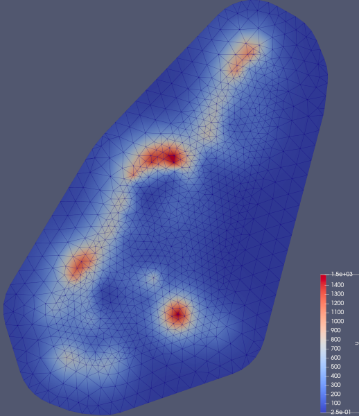

And the posterior standard deviation looks like this: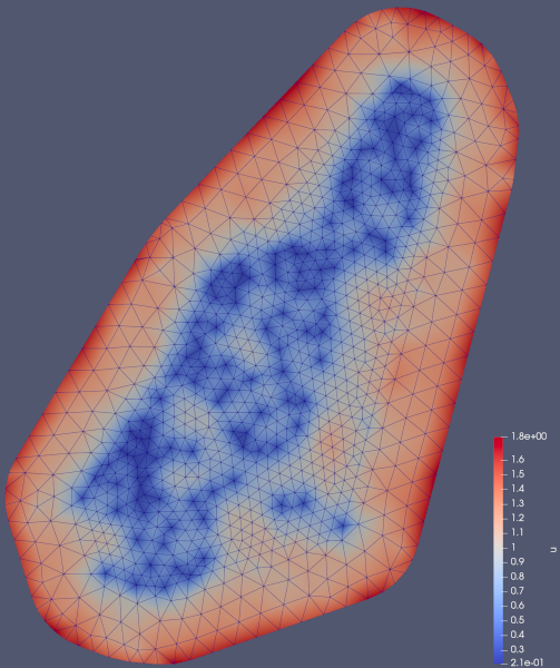

Final note

We have seen how to combine the modelling power of GPs with the efficiency of GMRFs. This is a powerful combination that allows us to model spatial data efficiently and accurately. Note that these models are still sensitive to the choice of hyperparameters, i.e. the range and smoothness of the Matern process. So it's quite likely that you may find better hyperparameters than the ones used in this tutorial.

This page was generated using Literate.jl.