Modelling on manifolds

Lots of interesting data does not live on a flat Euclidean domain. Global temperature measurements, satellite remote sensing products, and geomagnetic observations all live on (a sphere around) the Earth. A tempting shortcut is to treat longitude and latitude as planar coordinates and use standard spatial models. But this distorts distances badly near the poles, and the model produces artifacts at the dateline, where coordinates jump even though the physical domain is perfectly continuous there.

The SPDE approach [1] offers a principled way out. It defines a Matérn field as the solution of a stochastic PDE, and this definition carries over to (reasonably well-behaved) manifolds essentially unchanged: we simply replace the Laplacian with its manifold counterpart, the Laplace–Beltrami operator. Discretizing with finite elements on a mesh of the manifold then yields a GMRF — with all the sparse linear algebra machinery we know and love.

In this tutorial, we model data on the unit sphere. What it takes:

• A surface mesh of the sphere, which we build with Gmsh.

• A FEMDiscretization on that mesh — the elements are two-dimensional triangles, but their nodes have three-dimensional coordinates.

• That's it. MaternModel and friends work as usual from there.

Meshing the sphere

We use Gmsh's OpenCASCADE kernel to create a sphere and mesh its surface with triangles. FerriteGmsh then converts the result into a Ferrite grid.

using Ferrite, FerriteGmsh, Gmsh, LibGEOS
using GaussianMarkovRandomFields

function sphere_grid(mesh_size)
    Gmsh.initialize()
    gmsh.option.setNumber("General.Verbosity", 2)
    gmsh.model.add("sphere")
    gmsh.model.occ.addSphere(0.0, 0.0, 0.0, 1.0)
    gmsh.model.occ.synchronize()
    gmsh.option.setNumber("Mesh.MeshSizeMax", mesh_size)
    gmsh.model.mesh.generate(2)  ## 2 = mesh the surfaces only
    gmsh.model.mesh.renumberNodes()
    gmsh.model.mesh.renumberElements()
    nodes = FerriteGmsh.tonodes()
    elements, _ = FerriteGmsh.toelements(2)
    Gmsh.finalize()
    return Ferrite.Grid(elements, nodes)
end

grid = sphere_grid(0.1)

Grid{3, Triangle, Float64} with 3152 Triangle cells and 1578 nodes

The grid consists of triangles (reference dimension 2) whose nodes live in 3D space — a surface mesh embedded in 3D:

typeof(grid)

Grid{3, Triangle, Float64}

Let's look at it. We build a GeometryBasics.Mesh from the Ferrite grid once and reuse it for all sphere plots in this tutorial.

using CairoMakie
CairoMakie.activate!()
import GeometryBasics

points = [Point3f(n.x...) for n in grid.nodes]
triangles = [GeometryBasics.TriangleFace(Int.(c.nodes)...) for c in Ferrite.getcells(grid)]
sphere_mesh = GeometryBasics.Mesh(points, triangles)

fig = Figure(size = (500, 500))
ax = Axis3(fig[1, 1], aspect = :data, azimuth = 0.25π, title = "Sphere surface mesh")
hidedecorations!(ax)
hidespines!(ax)
wireframe!(ax, sphere_mesh, color = :steelblue, linewidth = 0.5)
fig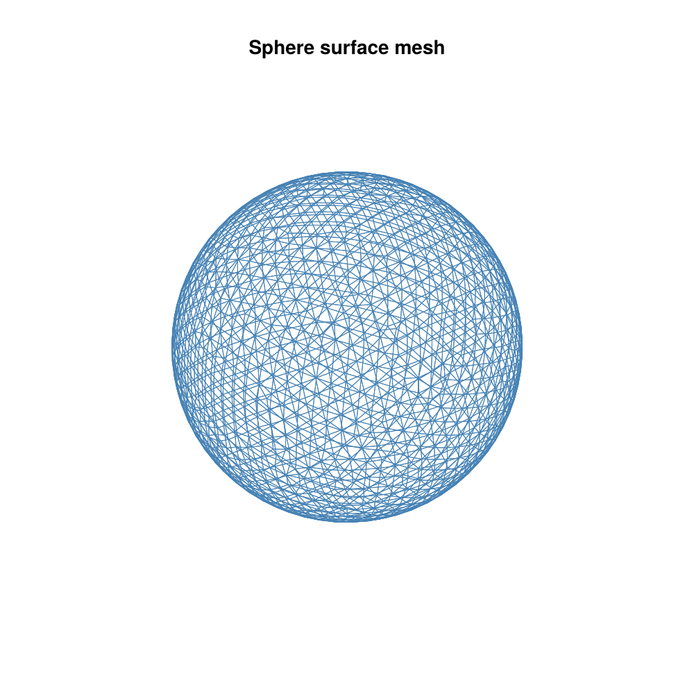

A Matérn field on the sphere

From here on, everything looks exactly like in the flat case: we build a FEMDiscretization and pass it to a MaternModel.

ip = Lagrange{RefTriangle, 1}()
qr = QuadratureRule{RefTriangle}(2)
disc = FEMDiscretization(grid, ip, qr)

FEMDiscretization
  grid: Grid{3, Triangle, Float64} with 3152 Triangle cells and 1578 nodes
  interpolation: Lagrange{RefTriangle, 1}()
  quadrature_rule: QuadratureRule{RefTriangle, Vector{Float64}, Vector{Vec{2, Float64}}}
  # constraints: 0

One thing deserves attention, though. The discretization now has two notions of dimension: the ambient dimension of the coordinates and the intrinsic dimension of the manifold.

ndim(disc), intrinsic_dim(disc)

(3, 2)

The distinction matters statistically: the relation $\alpha =\nu +d/2$ between the SPDE order and the Matérn smoothness, as well as the variance normalization, involve the dimension $d$ of the domain the field lives on — the intrinsic dimension 2, not the ambient dimension 3. GaussianMarkovRandomFields.jl handles this automatically.

We can now instantiate a Matérn field on the sphere and draw a sample from it. Note that the range parameter is measured in geodesic units — on the unit sphere, a range of 1 corresponds to about 57 degrees of arc.

using Random
model = MaternModel(disc; smoothness = 1)
u = model(τ = 1.0, range = 1.0)

rng = MersenneTwister(20)
s = rand(rng, u)

1578-element Vector{Float64}:
  0.055716930529207634
 -0.21043530882823913
  0.026898437971591055
 -1.2312889459132201
 -1.4010006573066094
 -1.243945285268592
 -0.2687384471273268
 -0.14715044607895547
 -0.1953384381006277
  0.16625610519944328
  ⋮
 -0.020920845384486977
 -0.9776424257778649
  0.10846677178059085
 -0.24827120434977124
  0.6335647342403921
 -0.8480363731925107
  1.065451725850944
 -0.979800145093953
 -0.3971208407638226

To color the surface by field values, we map the FEM coefficients to the mesh nodes. For first-order elements this is just a selection of the right degrees of freedom, which node_selection_matrix provides:

S = node_selection_matrix(disc, 1:Ferrite.getnnodes(grid))

fig = Figure(size = (600, 500))
ax = Axis3(fig[1, 1], aspect = :data, azimuth = 0.25π, title = "A Matérn sample on the sphere")
hidedecorations!(ax)
hidespines!(ax)
plt = mesh!(ax, sphere_mesh, color = S * s, colormap = :balance, shading = NoShading)
Colorbar(fig[1, 2], plt)
fig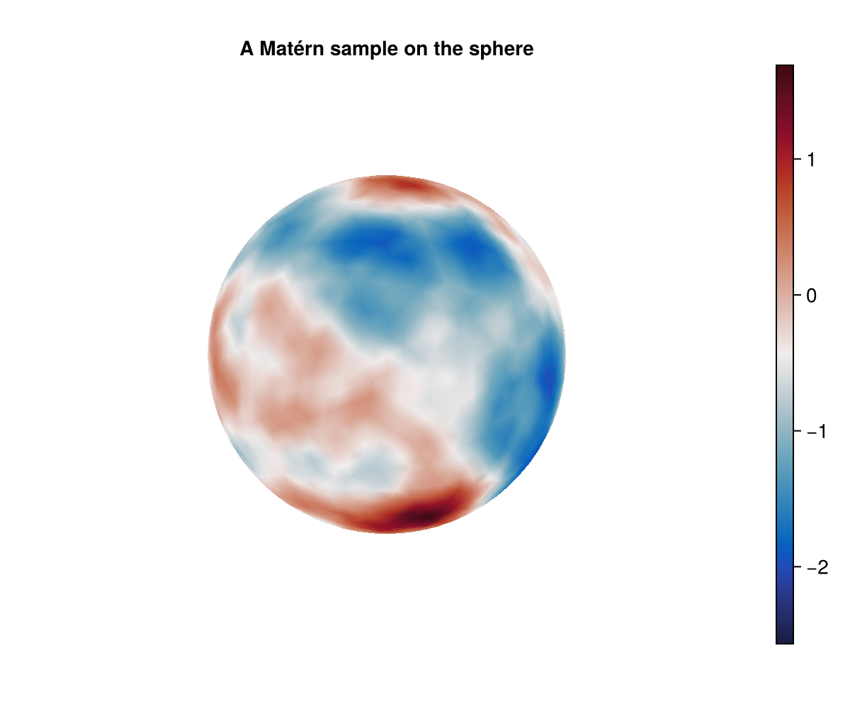

A smooth random field, with no seams and no polar artifacts — the sphere has no boundary, so there are no boundary effects either.

Sanity check: comparing against the exact solution

On the sphere we can do something that is rarely possible: check the GMRF against the exact solution of the SPDE. Expanding in spherical harmonics, the covariance of the Matérn SPDE solution between two points with angle $\theta$ between them is the series

$$C(\theta )=\sum _{l=0}^{\infty }\frac{2l+1}{4\pi }({\kappa }^2+l(l+1){)}^{-\alpha }{P}_l(\cos \theta ),$$

where $P_l$ are the Legendre polynomials. Let's implement this series with the classic three-term recurrence:

function sphere_matern_cov(costheta, κ, α; lmax = 2000)
    Plm1, Pl = one(costheta), costheta
    s = (1 / (4π)) * (κ^2)^(-α)
    s += (3 / (4π)) * (κ^2 + 2)^(-α) * costheta
    for l in 2:lmax
        Plp = ((2l - 1) * costheta * Pl - (l - 1) * Plm1) / l
        Plm1, Pl = Pl, Plp
        s += ((2l + 1) / (4π)) * (κ^2 + l * (l + 1))^(-α) * Pl
    end
    return s
end

sphere_matern_cov (generic function with 1 method)

Our model uses smoothness = 1, which on a 2D manifold means $\nu =2$ and $\alpha =\nu +d/2=3$, and range = 1.0 translates to $\kappa =\sqrt{8\nu }=4$. We compute the correlation function of the GMRF empirically — one column of the covariance matrix, obtained by a single sparse solve — and compare.

using LinearAlgebra, SparseArrays

Q = precision_matrix(model; τ = 1.0, range = 1.0)
ref_node = 1
ref_dof = findfirst(!iszero, S[ref_node, :])
e = zeros(size(Q, 1))
e[ref_dof] = 1.0
cov_column = cholesky(sparse(Q)) \ e
corr_fem = (S * cov_column) ./ cov_column[ref_dof]

1578-element Vector{Float64}:
 1.0
 0.0010270722480603942
 0.0010577730295321939
 0.0011468239034982059
 0.0012962207269772846
 0.0015236392748455983
 0.0018469108102867962
 0.002291766837074088
 0.0028943459800051946
 0.0037030846648890598
 ⋮
 0.1327565658548481
 0.010107649879090424
 0.2506737831845728
 0.01885355407957803
 0.17956296400995894
 0.008749960685851326
 0.03160988034402973
 0.047827592282788774
 0.014626091262588493

The angle between the reference node and every other node:

x_ref = grid.nodes[ref_node].x
angles = [acos(clamp(x_ref ⋅ n.x / (norm(x_ref) * norm(n.x)), -1, 1)) for n in grid.nodes]

1578-element Vector{Float64}:
 0.0
 3.141592653589793
 3.0434178831651124
 2.945243112740432
 2.847068342315751
 2.7488935718910708
 2.65071880146639
 2.5525440310417085
 2.4543692606170278
 2.3561944901923466
 ⋮
 1.0603887863277053
 1.9846510752822306
 0.8145310105246211
 1.762233162156182
 0.9475741693740486
 2.0370003117395976
 1.5804173625527773
 1.4315094491813734
 1.8541023159448786

For reference, we also include the Euclidean Matérn correlation evaluated at the geodesic distance — the "naive" formula one might be tempted to use.

using SpecialFunctions
ν, κ = 2, 4.0
euclidean_matern(d) = d ≈ 0 ? 1.0 : (2.0^(1 - ν) / gamma(ν)) * (κ * d)^ν * besselk(ν, κ * d)

θs = range(0, π, length = 200)
corr_exact = sphere_matern_cov.(cos.(θs), κ, 3) ./ sphere_matern_cov(1.0, κ, 3)

fig = Figure(size = (650, 400))
ax = Axis(
    fig[1, 1], xlabel = "Geodesic angle θ", ylabel = "Correlation",
    title = "GMRF vs. exact SPDE solution on the sphere",
)
scatter!(
    ax, angles, corr_fem, markersize = 3, color = (:steelblue, 0.3),
    label = "GMRF (FEM)",
)
lines!(ax, θs, corr_exact, color = :black, linewidth = 2, label = "Exact (spherical harmonics)")
lines!(
    ax, θs, euclidean_matern.(θs), color = :crimson, linewidth = 2,
    linestyle = :dash, label = "Euclidean Matérn at geodesic distance",
)
axislegend(ax)
fig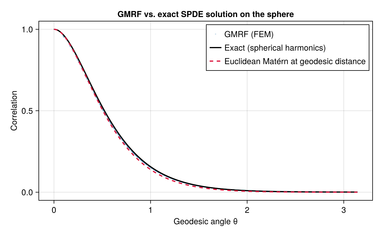

The GMRF matches the exact spherical solution. The Euclidean formula is a decent approximation here at short distances — the sphere looks locally flat — but the two visibly part ways at larger angles.

A small caveat in the same spirit: the variance normalization that makes σ² = 1 in MaternModel uses the Euclidean Matérn variance formula, which is only approximate on a curved manifold. On the sphere, the exact marginal variance of our field is

sphere_matern_cov(1.0, κ, 3) / (gamma(ν) / (gamma(ν + 1) * 4π * κ^(2ν)))

1.0433104436297547

— about 1% above the Euclidean value at this range. The discrepancy grows with the range, so keep it in mind when fields have ranges comparable to the radius of the sphere.

Conditioning on observations

Of course, we rarely just want to admire prior samples — we want to learn a field from data. Nothing about observations is specific to the manifold setting: we build a point-evaluation observation model, form the posterior, and plot it. Observation locations may be anywhere on the sphere — under the hood, they are projected onto the surface mesh.

Let's treat the sample s from before as the ground truth, observe it at 75 random locations with noise, and reconstruct it.

import Distributions

N_obs = 75
obs_points = [normalize(randn(rng, 3)) for _ in 1:N_obs]
A_obs = evaluation_matrix(disc, [Ferrite.Vec(p...) for p in obs_points])
σ_noise = 0.1
y = A_obs * s .+ σ_noise .* randn(rng, N_obs)

obs_matrix = permutedims(hcat(obs_points...))  ## N × 3 matrix of locations
obs_model = PointEvaluationObsModel(disc, obs_matrix, Distributions.Normal)
obs_lik = obs_model(y; σ = σ_noise)
u_posterior = gaussian_approximation(u, obs_lik)

fig = Figure(size = (1000, 450))
ax1 = Axis3(fig[1, 1], aspect = :data, azimuth = 0.25π, title = "Posterior mean")
hidedecorations!(ax1)
hidespines!(ax1)
plt = mesh!(ax1, sphere_mesh, color = S * mean(u_posterior), colormap = :balance, shading = NoShading)
scatter!(ax1, [Point3f(1.02 .* p...) for p in obs_points], color = :black, markersize = 5)
Colorbar(fig[1, 2], plt)
ax2 = Axis3(fig[1, 3], aspect = :data, azimuth = 0.25π, title = "Posterior std")
hidedecorations!(ax2)
hidespines!(ax2)
plt2 = mesh!(ax2, sphere_mesh, color = S * std(u_posterior), colormap = :viridis, shading = NoShading)
scatter!(ax2, [Point3f(1.02 .* p...) for p in obs_points], color = :white, markersize = 5)
Colorbar(fig[1, 4], plt2)
fig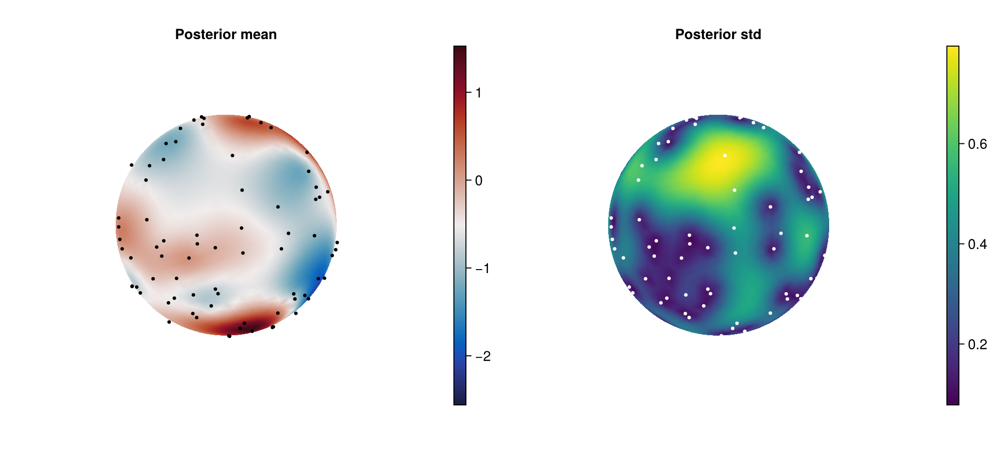

The posterior mean recovers the large-scale structure of the truth, and the posterior standard deviation dips around the observation locations (black / white dots) — just as it should.

Advection–diffusion on the sphere

Finally, let's turn up the fun and put dynamics on the sphere. The advection–diffusion SPDE of [2] describes a spatiotemporal field that is transported by a velocity field $\gamma$, diffuses, and is continually excited by spatially correlated noise.

On a manifold, the velocity field should be tangential. For the sphere, a natural choice is solid-body rotation about the $z$-axis, $\gamma (x)=\omega \times x$, which is tangential everywhere. We can pass exactly this function as the advection velocity:

ω = [0.0, 0.0, 2π / 3]  ## rotates by 120° per unit of time
wind(x) = Ferrite.Vec(
    ω[2] * x[3] - ω[3] * x[2],
    ω[3] * x[1] - ω[1] * x[3],
    ω[1] * x[2] - ω[2] * x[1],
)

ts = range(0.0, 1.0, length = 33)
adv_spde = AdvectionDiffusionSPDE{2}(
    κ = 0.1,
    α = 1 // 1,
    H = sparse(0.01 * I, 2, 2),  ## small diffusivity, expanded to 3D internally
    γ = wind,
    c = 1.0,
    τ = 0.1,
)
X = discretize(adv_spde, disc, ts)

MetaGMRF{ImplicitEulerMetadata}
  Inner GMRF: GMRF{Float64}(n=52074, alg=LinearSolve.DefaultLinearSolver)
  Metadata: ImplicitEulerMetadata{3}(1578 spatial × 33 time)

This is a GMRF over all length(ts) time slices jointly. We now observe a Gaussian bump on the equator at the initial time only and look at how the posterior mean evolves.

p0 = [1.0, 0.0, 0.0]
bump(p) = exp(-acos(clamp(p ⋅ p0, -1, 1))^2 / (2 * 0.4^2))

N_bump_obs = 300
bump_points = [normalize(randn(rng, 3)) for _ in 1:N_bump_obs]
y_bump = [bump(p) for p in bump_points] .+ 0.05 .* randn(rng, N_bump_obs)

A_spatial = evaluation_matrix(disc, [Ferrite.Vec(p...) for p in bump_points])
A_bump = spatial_to_spatiotemporal(A_spatial, 1, length(ts))
Q_noise = sparse(I, N_bump_obs, N_bump_obs) / 0.05^2
X_posterior = linear_condition(X; A = A_bump, Q_ϵ = Q_noise, y = y_bump)

means = time_means(X_posterior)

fig = Figure(size = (1000, 320))
crange = (-0.15, 1.0)
for (k, t_idx) in enumerate([1, 17, 33])
    local ax = Axis3(
        fig[1, k], aspect = :data, azimuth = 0.25π, elevation = 0.15π,
        title = "t = $(round(ts[t_idx], digits = 2))",
    )
    hidedecorations!(ax)
    hidespines!(ax)
    mesh!(
        ax, sphere_mesh, color = S * means[t_idx], colormap = :thermal,
        colorrange = crange, shading = NoShading,
    )
end
Colorbar(fig[1, 4], colorrange = crange, colormap = :thermal)
fig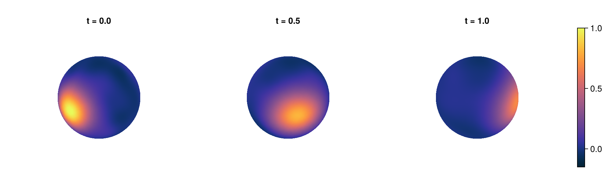

The reconstructed bump is carried eastward around the sphere by the rotation field, spreading out a little as it goes — advection and diffusion, live on a manifold. Even though we only observed the initial time, the dynamics encoded in the prior propagate that information across the whole spatiotemporal domain.

Closing remarks

Nothing in this tutorial was specific to the sphere: any triangulated surface embedded in 3D works the same way, as long as it is a reasonable discretization of a smooth manifold. And it composes with the rest of the package — non-Gaussian likelihoods, hyperparameter optimization through automatic differentiation, and hard linear constraints work on manifolds, too.

Two things to keep in mind:

• Hyperparameters are measured in geodesic units of the manifold — for the Earth, remember to work on a sphere of the appropriate radius (or rescale your ranges).

• The σ² = 1 variance normalization is exact in Euclidean space and slightly approximate on curved manifolds, as we quantified above.

---

This page was generated using Literate.jl.