Bernoulli Spatial Classification with a Matérn Field

In this walkthrough you will build a simple probabilistic classifier for spatial point data with binary labels. We combine:

• a spatial latent Gaussian field with a Matérn covariance (via SPDE), and

• a Bernoulli observation model with a logit link for classification.

You will learn how to:

• construct a Matérn latent model from coordinates,

• connect it to Bernoulli observations,

• perform a fast Gaussian approximation to the posterior, and

• make and visualize spatial probability predictions on a grid.

Written out, the model is

$$u\sim \mathcal{GP}(0,k_{\nu }(\cdot ,\cdot )),y_i\mid u\sim \mathrm{Bernoulli}(p(s_i)),\mathrm{logit}p(s_i)=u(s_i),$$

where $u$ is a Matérn field with smoothness $\nu$, approximated by a GMRF through its SPDE representation, and $s_i$ are the observed locations. The logit link keeps $p(s_i)\in (0,1)$ without constraining $u$.

The posterior $p(u\mid y)$ is not Gaussian, because the Bernoulli likelihood is not conjugate to the prior. We approximate it by the Gaussian centred at the posterior mode with matching curvature — the Laplace approximation — which gaussian_approximation computes.

We use the well-known Lansing Woods dataset (tree locations with species marks). The dataset here provides three columns: x, y, is_hickory (0/1). We try a local file first so the tutorial works offline; otherwise we download a small RDA file from the upstream repository.

using DataFrames
using GaussianMarkovRandomFields

Loading the FEM weakdeps activates the GaussianMarkovRandomFieldsFEM extension which provides MaternModel and the underlying SPDE machinery.

using Ferrite, FerriteGmsh, Gmsh, LibGEOS
using LinearAlgebra, Random
using Plots

Load data (local if present, otherwise download)

using CodecBzip2, RData
data_dir = joinpath(@__DIR__, "data")
mkpath(data_dir)
local_rda = joinpath(data_dir, "lansing_trees.rda")

if !isfile(local_rda)
    repo_url = "https://github.com/spatstat/spatstat.data/raw/refs/heads/master/data/lansing.rda"
    try
        download(repo_url, local_rda)
    catch err
        error(
            "Could not download dataset (are you offline?). " *
                "Place an RData file at $(local_rda) or pass your own DataFrame."
        )
    end
end

objs = RData.load(local_rda)["lansing"]
x, y = objs[objs.name2index["x"]], objs[objs.name2index["y"]]
is_hickory = objs[objs.name2index["marks"]] .== "hickory"

df = DataFrame(["x" => x, "y" => y, "is_hickory" => is_hickory])
df = unique(df)  # remove any accidental duplicates
first(df, 5)     # show a preview in the docs

5×3 DataFrame

Row	x	y	is_hickory
	Float64	Float64	Bool
1	0.078	0.091	false
2	0.076	0.266	false
3	0.051	0.225	false
4	0.015	0.366	false
5	0.03	0.426	false

Coordinates and binary label (1=hickory, 0=other)

X = Matrix(df[:, [:x, :y]])
y = Vector{Int}(df[:, :is_hickory])

2250-element Vector{Int64}:
 0
 0
 0
 0
 0
 0
 0
 0
 0
 0
 ⋮
 0
 0
 0
 0
 0
 0
 0
 0
 0

Train/test split

We take a random 80/20 split for a quick, reproducible evaluation.

Random.seed!(42)
n = size(X, 1)
perm = randperm(n)
split = round(Int, 0.8n)
train_idcs = perm[1:split]
test_idcs = perm[(split + 1):end]

X_train, y_train = X[train_idcs, :], y[train_idcs]
X_test, y_test = X[test_idcs, :], y[test_idcs]

([0.497 0.562; 0.756 0.793; … ; 0.718 0.411; 0.17 0.085], [0, 0, 0, 0, 0, 0, 0, 0, 1, 1  …  1, 0, 1, 1, 0, 0, 0, 0, 0, 0])

Latent model: Matérn GP via SPDE

We construct a spatial latent model from the observation coordinates. Under the hood this builds a sparse SPDE representation of a Matérn Gaussian field.

Key hyperparameters:

• smoothness: controls differentiability of the field. We use 1 by default which is a common choice for spatial classification.

• range: controls the distance over which the field exhibits strong correlation. As a rule of thumb, set it to a fraction of the spatial extent of your data.

latent = MaternModel(X; smoothness = 1)
u = latent(τ = 1.0, range = 0.2)  # tune this to your dataset's scale

GMRF{Float64} with 8321 variables
  Algorithm: LinearSolve.CHOLMODFactorization{Nothing}
  Mean: [0.0, 0.0, 0.0, ..., 0.0, 0.0, 0.0]
  Q_sqrt: not available

Bernoulli observations (logit link)

We connect the latent field to point-wise labels using a Bernoulli exponential family model with a logit link. The model is evaluated at the observed locations.

import Distributions
obs_model = PointEvaluationObsModel(latent.discretization, X_train, Distributions.Bernoulli)
lik = obs_model(y_train)

LinearlyTransformedLikelihood{BernoulliLikelihood{LogitLink, Nothing}, SparseArrays.SparseMatrixCSC{Float64, Int64}, Nothing}(BernoulliLikelihood{LogitLink, Nothing}(LogitLink(), [1, 0, 0, 1, 0, 1, 1, 1, 0, 0  …  0, 0, 1, 0, 0, 0, 1, 1, 0, 0], nothing), sparse([1150, 1737, 1737, 1737, 1544, 1544, 1544, 84, 84, 84  …  540, 416, 1777, 1198, 212, 1691, 1137, 1712, 1110, 884], [1, 4, 5, 6, 7, 8, 9, 10, 11, 12  …  8263, 8265, 8271, 8272, 8283, 8286, 8292, 8294, 8304, 8311], [3.1086244689504383e-15, 1.0, 0.0, 8.326672684688674e-16, 0.0, 0.0, 1.0, 1.0, 0.0, 2.220446049250313e-16  …  0.999999999999996, 1.0, 0.9999999999999938, 1.0, 1.0, 1.0, 1.0, 0.9999999999999927, 1.0, 0.9999999999999942], 1800, 8321), nothing)

Inference: Gaussian approximation

We perform a Gaussian approximation of the posterior for the latent field u given the Bernoulli observations. This is typically very fast thanks to the sparse structure of the SPDE discretization.

post = gaussian_approximation(u, lik)

GMRF{Float64} with 8321 variables
  Algorithm: LinearSolve.CHOLMODFactorization{Nothing}
  Mean: [0.33076627906835043, 0.04608798195131945, 0.016746075149262445, ..., 0.5858919787370958, 0.8286802673225974, -0.2802355906234742]
  Q_sqrt: not available

Evaluation on held-out data

To score the classifier we predict probabilities at test locations. The helper conditional_distribution returns the predictive distribution of the linear predictor at new points; taking mean applies the Bernoulli mean transform under the logit link to yield probabilities in [0,1].

obs_model_test = PointEvaluationObsModel(latent.discretization, X_test, Distributions.Bernoulli)
pred_dist_test = conditional_distribution(obs_model_test, mean(post))

Distributions.Product{Distributions.Discrete, Distributions.Bernoulli{Float64}, Vector{Distributions.Bernoulli{Float64}}}(
v: Distributions.Bernoulli{Float64}[Distributions.Bernoulli{Float64}(p=0.21028351261511163), Distributions.Bernoulli{Float64}(p=0.26762843729656693), Distributions.Bernoulli{Float64}(p=0.3838347617465545), Distributions.Bernoulli{Float64}(p=0.26066824677517325), Distributions.Bernoulli{Float64}(p=0.21088389188294032), Distributions.Bernoulli{Float64}(p=0.3637381198287554), Distributions.Bernoulli{Float64}(p=0.585830457114353), Distributions.Bernoulli{Float64}(p=0.14389922222761212), Distributions.Bernoulli{Float64}(p=0.24316534828350553), Distributions.Bernoulli{Float64}(p=0.5448418290004261)  …  Distributions.Bernoulli{Float64}(p=0.4461312217836382), Distributions.Bernoulli{Float64}(p=0.16047205782238785), Distributions.Bernoulli{Float64}(p=0.6760532623331568), Distributions.Bernoulli{Float64}(p=0.2927339087876812), Distributions.Bernoulli{Float64}(p=0.20438185924482954), Distributions.Bernoulli{Float64}(p=0.0651174661254955), Distributions.Bernoulli{Float64}(p=0.31011935615659375), Distributions.Bernoulli{Float64}(p=0.2605072380879234), Distributions.Bernoulli{Float64}(p=0.40201964396369516), Distributions.Bernoulli{Float64}(p=0.11953858361257662)]
)

Convert to probabilities and class labels (0/1) using a 0.5 threshold.

ŷ_prob = mean(pred_dist_test)  # probability for class "hickory"
ŷ = Int.(ŷ_prob .>= 0.5)

accuracy = sum(ŷ .== y_test) / length(y_test)
accuracy

0.74

Visualization

A simple heatmap of predicted probabilities with all observed points overlaid. Redder areas indicate higher probability of class "hickory".

xmin, xmax = extrema(X[:, 1])
ymin, ymax = extrema(X[:, 2])
nx, ny = 100, 100
xs = range(xmin, xmax; length = nx)
ys = range(ymin, ymax; length = ny)

grid_points = Array{Float64}(undef, nx * ny, 2)
for (i, (yv, xv)) in enumerate(Iterators.product(ys, xs))
    grid_points[i, 1] = xv
    grid_points[i, 2] = yv
end

obs_grid = PointEvaluationObsModel(latent.discretization, grid_points, Distributions.Bernoulli)
pred_grid = conditional_distribution(obs_grid, mean(post))
probs = reshape(mean(pred_grid), (nx, ny))

plt = heatmap(
    xs, ys, probs; xlabel = "x", ylabel = "y",
    title = "P(is_hickory=1) — acc=$(round(accuracy, digits = 3))",
    colorbar = true, legend = :topright
)

class0 = findall(==(0), y)
class1 = findall(==(1), y)

scatter!(plt, X[class1, 1], X[class1, 2]; m = :circle, ms = 1.5, c = :tomato, label = "hickory")
scatter!(plt, X[class0, 1], X[class0, 2]; m = :circle, ms = 1.5, c = :royalblue, label = "other")
plt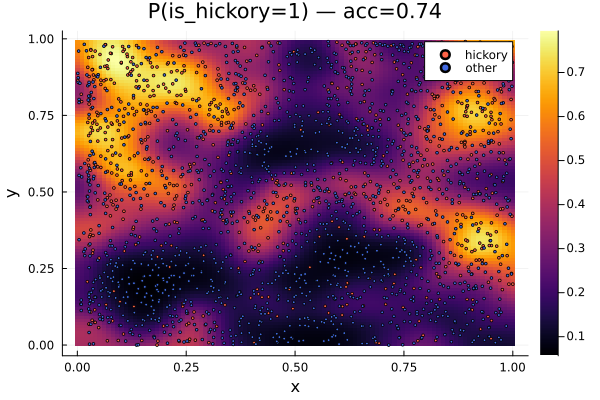

Notes and tips

• Hyperparameters matter: start by adjusting range so the spatial field varies on a scale similar to your data. If predictions look too smooth or too noisy, increase or decrease range respectively.

• Performance scales well: the SPDE discretization yields sparse matrices, making inference and prediction efficient for thousands to millions of points.

• Your own data: if you already have a DataFrame with columns :x, :y, and a boolean/0-1 label column, set df accordingly and keep the rest unchanged.

• Offline runs: if the download step fails, add your file at docs/src/literate-tutorials/data/lansing_trees.rda or point df to your data.

---

This page was generated using Literate.jl.