
Getting started
Nearly every workflow in this package has the same three steps. First we choose a latent model, which says what we expect the unknown field to look like before seeing any data. Then we choose an observation model, which relates that field to the data. Finally we compute the posterior.
We go through those steps twice below: once on a time series, using nothing but the package itself, and once on a spatial problem, where a handful of extra packages buy us a considerably richer prior. The spatial example is the one you are more likely to adapt for your own work. The first one exists to show what happens underneath.
A time series
The AR(1) process is about the smallest GMRF worth writing down. AR1Model fixes the structure – 200 time points, each one correlated with its predecessor – without committing to parameter values yet.
using GaussianMarkovRandomFields
using Distributions, LinearAlgebra, SparseArrays, Random
using Plots

Random.seed!(2)

N = 200
model = AR1Model(N)
hyperparameters(model)
(τ = Real, ρ = Real)Supplying those hyperparameters turns the model into an actual distribution. τ is a precision, so larger values mean less variation, and ρ sets the correlation between neighbouring time points.
prior = model(τ = 1.0, ρ = 0.95)GMRF{Float64} with 200 variables
Algorithm: LinearSolve.LDLtFactorization{Nothing}
Mean: [0.0, 0.0, 0.0, ..., 0.0, 0.0, 0.0]
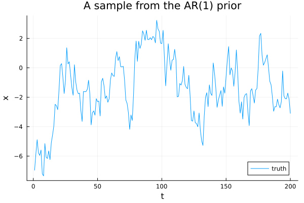
Q_sqrt: not availableThe result behaves like any other Distributions.jl distribution. Let us draw a sample and treat it as the ground truth we are going to try to recover.
x_true = rand(prior)
plot(
    x_true, label = "truth", xlabel = "t", ylabel = "x",
    title = "A sample from the AR(1) prior"
)
What makes this a GMRF rather than just a Gaussian is the precision matrix. For an AR(1) model it is tridiagonal, because each time point interacts only with its immediate neighbours – so much so that the package stores it in a dedicated tridiagonal type rather than as a general sparse matrix:
Q = to_matrix(precision_map(prior))
typeof(Q)
LinearAlgebra.SymTridiagonal{Float64, Vector{Float64}}Either way, only a vanishing fraction of the entries are nonzero:
"$(count(!iszero, Q)) nonzeros out of $(length(Q)) entries""598 nonzeros out of 40000 entries"That is the whole trick. The covariance matrix of this distribution is completely dense, but we never form it – everything is computed from the sparse precision instead.
Observations
Suppose we only get to see the process at 15 time points, corrupted by independent Gaussian noise. Written as a linear model, that is
obs_idcs = sort(randperm(N)[1:15])
A = sparse(1:length(obs_idcs), obs_idcs, 1.0, length(obs_idcs), N)

σ_noise = 0.3
y = A * x_true .+ σ_noise .* randn(length(obs_idcs))
15-element Vector{Float64}:
-4.975305937722804
-5.951375015608471
-1.8526121978345638
-0.8534502270612697
-0.05469935873430981
0.11770925778542318
-0.5877273034403836
-3.993460891574649
-0.341128043302585
1.6706347724257309
-1.8239216716361861
1.997398230017473
0.5548397350225491
-2.2740024873209657
-3.4710521716573033linear_condition conditions the prior on exactly this kind of linear observation. The noise enters as a precision, so we pass 1 / σ².
posterior = linear_condition(prior; A = A, Q_ϵ = (1 / σ_noise^2) * I, y = y)GMRF{Float64} with 200 variables
Algorithm: LinearSolve.DefaultLinearSolver
Mean: [-4.477324578596489, -4.712973240627884, -4.961024463818826, ..., -2.839079201812524, -3.1304221212302674, -3.430002993598616]
Q_sqrt: not availableThe posterior is another GMRF, so mean and std work as before. Plotting the mean with a two-standard-deviation band shows the field being pinned down near the observations and reverting to the prior away from them.
post_mean = mean(posterior)
post_std = std(posterior)

plot(
    post_mean, ribbon = 2 * post_std, label = "posterior mean ± 2σ",
    xlabel = "t", ylabel = "x", title = "AR(1) posterior"
)
plot!(x_true, label = "truth", linestyle = :dash)
scatter!(obs_idcs, y, label = "observations", markersize = 3)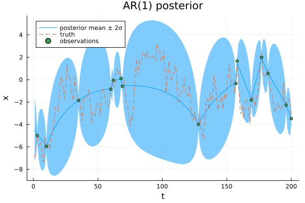
A spatial field
Time series are easy because we can write the precision matrix down by hand. In space that is much harder, and it is where the SPDE approach comes in: a Matérn Gaussian process can be characterised as the solution of a stochastic partial differential equation, and discretizing that equation with finite elements yields a GMRF that approximates it. [1] worked out the details; the package hides them.
The finite element machinery lives in a package extension, which activates once all four of these are loaded:
using Ferrite, FerriteGmsh, Gmsh, LibGEOSWe scatter some observation locations in the plane and let MaternModel build a mesh and a discretization around them. smoothness is the Matérn parameter ν, as an integer.
Random.seed!(3)
n_obs = 60
points = rand(n_obs, 2)

matern = MaternModel(points; smoothness = 1)
spatial_prior = matern(τ = 1.0, range = 0.3)
GMRF{Float64} with 366 variables
Algorithm: LinearSolve.CHOLMODFactorization{Nothing}
Mean: [0.0, 0.0, 0.0, ..., 0.0, 0.0, 0.0]
Q_sqrt: not availableSynthetic observations of a smooth function, again with Gaussian noise:
f(x, y) = sin(2π * x) * cos(2π * y)
y_spatial = [f(points[i, 1], points[i, 2]) for i in 1:n_obs] .+ 0.1 .* randn(n_obs)
60-element Vector{Float64}:
0.47535399769054787
-0.11990045264422194
-0.04203640824339096
0.045515338801003925
0.23055182515367387
-0.8094511656608449
-0.008151355124152593
-0.29001968584331755
-0.9165702100659167
-0.9241918255528857
⋮
-0.05673602107892754
0.0495038090796156
-0.8329674237636615
0.7281238455760184
-0.17833593272187853
-0.3011392072988227
-0.8147267694708649
0.0941164913391212
-0.8759454298390502This time we use the observation-model interface rather than assembling A ourselves. PointEvaluationObsModel knows how to evaluate the field at our points, and calling it with the data and a noise level produces a likelihood.
obs_model = PointEvaluationObsModel(matern, Normal)
likelihood = obs_model(y_spatial; σ = 0.1)

spatial_posterior = gaussian_approximation(spatial_prior, likelihood)
GMRF{Float64} with 366 variables
Algorithm: LinearSolve.CHOLMODFactorization{Nothing}
Mean: [0.7231777324617992, 0.45411206146091865, 0.4274828949947919, ..., -0.22579266399826595, -0.06647601160017877, 0.20299766713227174]
Q_sqrt: not availablegaussian_approximation is the general entry point for combining a prior with a likelihood. For a Gaussian likelihood such as this one the result is exact. For non-Gaussian likelihoods it returns the Laplace approximation instead, which is what the Bernoulli classification tutorial builds on.
Predicting on a grid
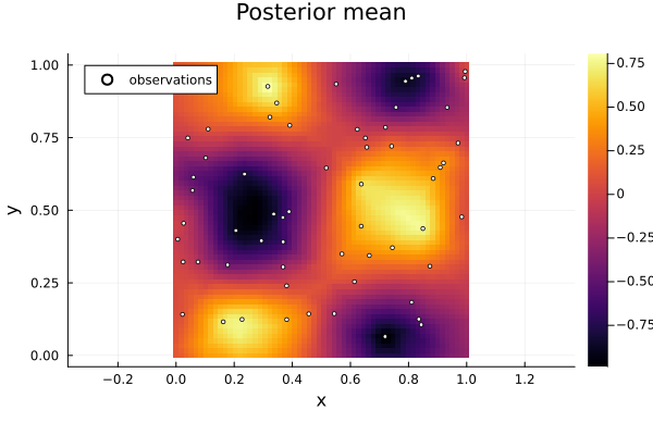
To see the fitted field we evaluate the posterior on a regular grid, which is once again a point evaluation – just at different locations.
ngrid = 60
gx = range(0, 1; length = ngrid)
gy = range(0, 1; length = ngrid)
grid_points = Array{Float64}(undef, ngrid^2, 2)
for (i, (yv, xv)) in enumerate(Iterators.product(gy, gx))
    grid_points[i, 1] = xv
    grid_points[i, 2] = yv
end

grid_obs = PointEvaluationObsModel(matern.discretization, grid_points, Normal)
pred = conditional_distribution(grid_obs, mean(spatial_posterior); σ = 0.1)
pred_mean = reshape(mean(pred), (ngrid, ngrid))

hm = heatmap(
    gx, gy, pred_mean, xlabel = "x", ylabel = "y",
    title = "Posterior mean", aspect_ratio = :equal
)
scatter!(
    hm, points[:, 1], points[:, 2], label = "observations",
    markersize = 2, color = :white, markerstrokecolor = :black
)
Where to go next
The tutorials are self-contained, so pick whichever is closest to your problem:
Building autoregressive models derives the AR(1) precision matrix above by hand, and is the place to start if the sparsity story is what interests you.
Spatial Modelling with SPDEs treats the spatial example properly, on real data, including how to choose hyperparameters.
Bernoulli Spatial Classification with a Matérn Field and Advanced GMRF modelling for disease mapping cover non-Gaussian observations.
Automatic Differentiation for GMRF Hyperparameters shows how to fit hyperparameters by gradient-based optimization rather than choosing them by hand.
This page was generated using Literate.jl.