
Automatic Differentiation and MCMC
Introduction
Gaussian Markov Random Fields (GMRFs) are powerful tools for Bayesian inference. When the parameters of a GMRF model are unknown, we often want to infer them from observed data. Traditional optimization methods can be limiting, but modern MCMC methods like NUTS (No-U-Turn Sampler) provide a robust approach for full Bayesian inference.
Automatic differentiation (AD) is crucial for efficient MCMC sampling, as it enables gradient-based samplers to explore complex posterior geometries effectively. This tutorial demonstrates how to leverage AD with GMRFs for Bayesian parameter inference using NUTS in Turing.jl.
AD support in GaussianMarkovRandomFields.jl works through custom chain rules that enable automatic differentiation through the linear algebra operations needed for GMRF computations.
using Distributions
using GaussianMarkovRandomFields
using Random, LinearAlgebra, SparseArrays
using Plots
MCMC Parameter Inference for CAR Models
We'll demonstrate Bayesian inference for the parameters of a conditional autoregressive (CAR) model. Given observations from a CAR process, we'll infer both the spatial correlation parameter (ρ) and variance parameter (σ) using NUTS sampling.
Problem setup: CAR model parameter inference
We'll tackle a simple 1D time series problem: given observations sampled from a conditional autoregressive (CAR) process, infer the CAR parameter (ρ).
using Turing, SparseArraysSet up a 1D grid (time points)
xs = 0:0.1:2  # 21 time points
N = length(xs)21Create adjacency matrix for second-order CAR (neighbors and next-neighbors)
W = spzeros(N, N)
for i in 1:N
    for k in [-2, -1, 1, 2]
        j = i + k
        if 1 <= j <= N
            W[i, j] = 1.0 / abs(k)
        end
    end
end
Generate synthetic observations from true CAR process
Random.seed!(123)
true_ρ = 0.85  # True CAR parameter
true_σ = 0.01  # True field variance
μ = zeros(N)   # Zero mean
21-element Vector{Float64}:
0.0
0.0
0.0
0.0
0.0
0.0
0.0
0.0
0.0
0.0
⋮
0.0
0.0
0.0
0.0
0.0
0.0
0.0
0.0
0.0Generate true CAR model and sample from it
true_car = generate_car_model(W, true_ρ; μ = μ, σ = true_σ)GMRF{Float64} with 21 variables
Algorithm: LinearSolve.DefaultLinearSolver
Mean: [0.0, 0.0, 0.0, ..., 0.0, 0.0, 0.0]
Q_sqrt: not availableOur "observations" are just a sample from the true CAR
observations = rand(true_car)

println("Generated observations from CAR process with $(N) time points")
println("True CAR parameter ρ: $(true_ρ)")
println("True variance parameter σ: $(true_σ)")
Generated observations from CAR process with 21 time points
True CAR parameter ρ: 0.85
True variance parameter σ: 0.01Bayesian model in Turing
We'll use a simple model:
x ~ CAR(W, ρ, σ) where ρ and σ are parameters to infer
ρ ~ Uniform(0.5, 0.99)
σ ~ Uniform(0.001, 0.1)
y = x (direct observation of the CAR process)
@model function car_model(y, W, μ)
    # Prior on CAR parameter
    ρ ~ Uniform(0.5, 0.99)

    # Prior on variance parameter
    σ ~ Uniform(0.001, 0.1)

    # CAR process
    car_dist = generate_car_model(W, ρ; μ = μ, σ = σ)

    # Direct observation
    y ~ car_dist
end
car_model (generic function with 2 methods)Create the model
model = car_model(observations, W, μ)DynamicPPL.Model{typeof(Main.car_model), (:y, :W, :μ), (), (), Tuple{Vector{Float64}, SparseArrays.SparseMatrixCSC{Float64, Int64}, Vector{Float64}}, Tuple{}, DynamicPPL.DefaultContext, false}(Main.car_model, (y = [0.07840387299483456, 0.08930313551294568, 0.05681030361934514, 0.08267097408818344, -0.025373176002426053, -0.052514495598035886, -0.16214702025581987, -0.05502378606163387, -0.05182846203947111, -0.011947395381926016 … 0.0163799355582178, 0.021789192443508004, -0.07393817365539637, -0.05328451077296107, -0.020084724732943475, 0.0006785820490446196, -0.03016630854446354, -0.08709273978627284, -0.13240380240329042, -0.033708664634961895], W = sparse([2, 3, 1, 3, 4, 1, 2, 4, 5, 2 … 20, 17, 18, 20, 21, 18, 19, 21, 19, 20], [1, 1, 2, 2, 2, 3, 3, 3, 3, 4 … 18, 19, 19, 19, 19, 20, 20, 20, 21, 21], [1.0, 0.5, 1.0, 1.0, 0.5, 0.5, 1.0, 1.0, 0.5, 0.5 … 0.5, 0.5, 1.0, 1.0, 0.5, 0.5, 1.0, 1.0, 0.5, 1.0], 21, 21), μ = [0.0, 0.0, 0.0, 0.0, 0.0, 0.0, 0.0, 0.0, 0.0, 0.0 … 0.0, 0.0, 0.0, 0.0, 0.0, 0.0, 0.0, 0.0, 0.0, 0.0]), NamedTuple(), DynamicPPL.DefaultContext())MCMC Sampling with NUTS
NUTS requires gradients, which are automatically computed thanks to our autodifferentiable GMRF implementation.
println("Starting MCMC sampling...")
Random.seed!(456)

sampler = NUTS()
chain = sample(model, sampler, 1000, progress = false)

println("MCMC sampling completed!")
Starting MCMC sampling...
┌ Info: Found initial step size
└ ϵ = 1.6
MCMC sampling completed!Analyze results
Extract CAR parameter samples
ρ_samples = chain[:ρ].data[:, 1]
ρ_mean = mean(ρ_samples)
ρ_std = std(ρ_samples)0.1223985768558768Extract variance parameter samples
σ_samples = chain[:σ].data[:, 1]
σ_mean = mean(σ_samples)
σ_std = std(σ_samples)

println("Posterior summary for CAR parameter ρ:")
println("True value: $(true_ρ)")
println("Posterior mean: $(round(ρ_mean, digits = 4)) ± $(round(ρ_std, digits = 4))")
println("95% credible interval: $(round(quantile(ρ_samples, 0.025), digits = 4)) - $(round(quantile(ρ_samples, 0.975), digits = 4))")

ρ_in_ci = quantile(ρ_samples, 0.025) <= true_ρ <= quantile(ρ_samples, 0.975)
println("True ρ value in 95% CI: $(ρ_in_ci)")

println("\nPosterior summary for variance parameter σ:")
println("True value: $(true_σ)")
println("Posterior mean: $(round(σ_mean, digits = 4)) ± $(round(σ_std, digits = 4))")
println("95% credible interval: $(round(quantile(σ_samples, 0.025), digits = 4)) - $(round(quantile(σ_samples, 0.975), digits = 4))")

σ_in_ci = quantile(σ_samples, 0.025) <= true_σ <= quantile(σ_samples, 0.975)
println("True σ value in 95% CI: $(σ_in_ci)")
Posterior summary for CAR parameter ρ:
True value: 0.85
Posterior mean: 0.7848 ± 0.1224
95% credible interval: 0.5301 - 0.9702
True ρ value in 95% CI: true
Posterior summary for variance parameter σ:
True value: 0.01
Posterior mean: 0.0095 ± 0.0035
95% credible interval: 0.0048 - 0.0184
True σ value in 95% CI: truePlot posterior for CAR parameter
p1 = histogram(
    ρ_samples, bins = 20, alpha = 0.7, label = "Posterior samples",
    xlabel = "CAR Parameter ρ", ylabel = "Density",
    title = "Posterior Distribution of ρ"
)
vline!([true_ρ], label = "True Value", color = :red, linewidth = 2)
vline!([ρ_mean], label = "Posterior Mean", color = :blue, linewidth = 2, linestyle = :dash)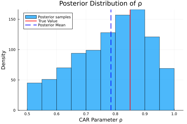
Plot posterior for variance parameter
p2 = histogram(
    σ_samples, bins = 20, alpha = 0.7, label = "Posterior samples",
    xlabel = "Variance Parameter σ", ylabel = "Density",
    title = "Posterior Distribution of σ"
)
vline!([true_σ], label = "True Value", color = :red, linewidth = 2)
vline!([σ_mean], label = "Posterior Mean", color = :blue, linewidth = 2, linestyle = :dash)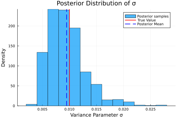
Plot trace of CAR parameter
p3 = plot(
    ρ_samples, label = "ρ samples", xlabel = "Iteration", ylabel = "CAR Parameter ρ",
    title = "MCMC Trace for ρ"
)
hline!([true_ρ], label = "True Value", color = :red, linewidth = 2)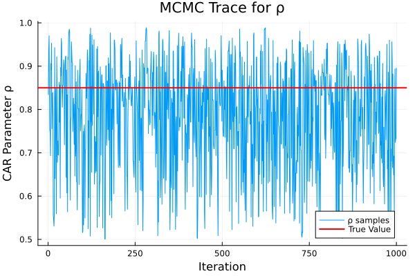
Plot trace of variance parameter
p4 = plot(
    σ_samples, label = "σ samples", xlabel = "Iteration", ylabel = "Variance Parameter σ",
    title = "MCMC Trace for σ"
)
hline!([true_σ], label = "True Value", color = :red, linewidth = 2)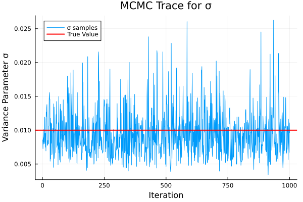
Combine plots
combined_plot = plot(p1, p2, p3, p4, layout = (2, 2), size = (1000, 800))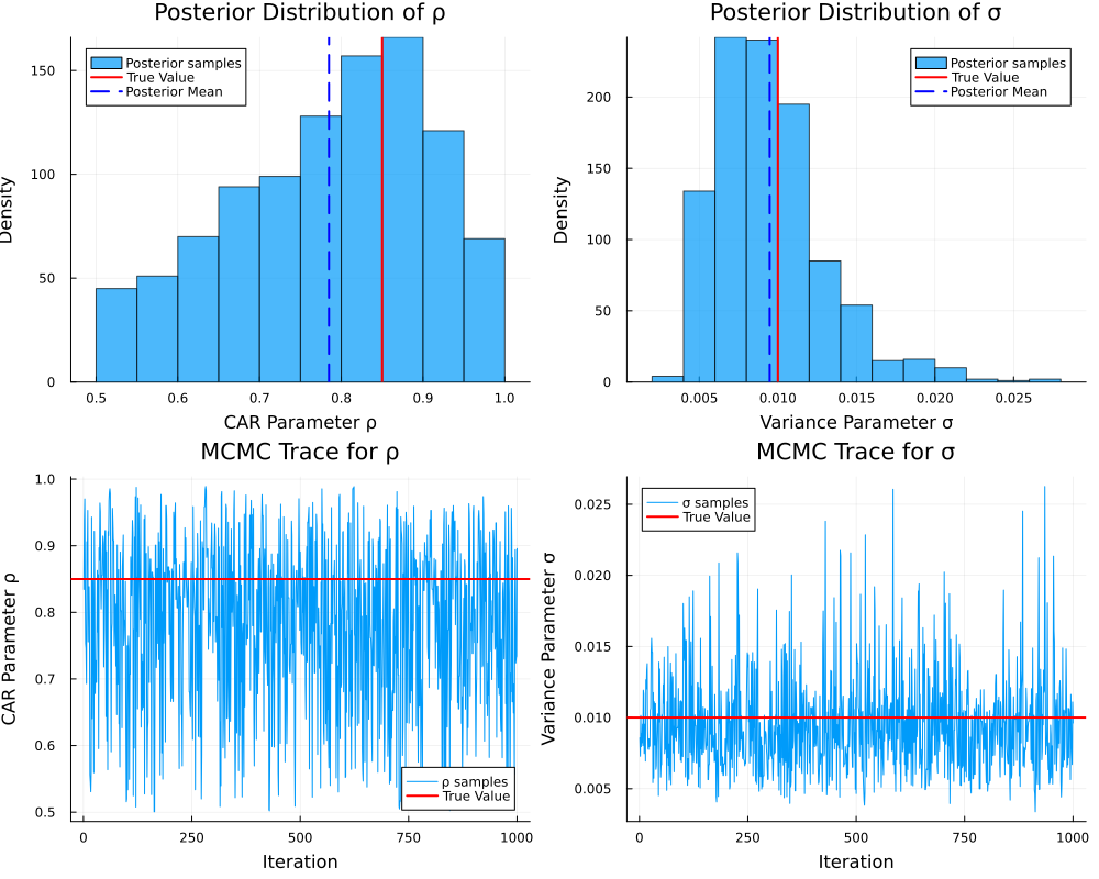
Conclusion
This tutorial demonstrated how AD enables advanced sampling methods like NUTS for full Bayesian inference with GMRFs.
In practice, MCMC still quickly becomes prohibitively expensive, so people instead use Integrated Nested Laplace Approximations (INLA). More on this soon.
This page was generated using Literate.jl.