
Advanced GMRF modelling for disease mapping
In this walk‑through we fit a simple, interpretable disease‑mapping model to the classic Scotland lip cancer data. The response is the number of observed cases per district. We use a Poisson likelihood with an exposure offset and a BYM (Besag–York–Mollié) latent field to capture spatial structure and local over‑dispersion. We also include a fixed‑effect covariate.
What we put together:
A Poisson model with a log link and log‑exposure offset (so we model relative risk).
A BYM latent field = Besag (structured spatial) + IID (unstructured spatial).
Fixed effects (intercept + one covariate).
In symbols, for district
so
where
What you’ll learn:
Build a polygon contiguity adjacency matrix directly from a shapefile.
Compose a BYM + fixed‑effects model via the formula interface.
Run a fast Gaussian approximation and make useful maps.
Read fixed effects, split BYM into structured/unstructured, and add an exceedance map (P(RR > 1)).
using CSV, DataFrames
using StatsModels
using SparseArrays
using Distributions
using GaussianMarkovRandomFields
using Shapefile              # Activates the Shapefile extension for contiguity
using LibGEOS
using Plots
using GeoInterface
using Random, Statistics
Load data
We load from a local data/ directory next to this tutorial. The CSV has observed counts (CANCER), expected counts (CEXP), and the covariate AFF: the proportion of the population engaged in Agriculture, Fishing or Forestry (hence the name). The shapefile contains district polygons with a CODE attribute. We align the CSV rows to the shapefile feature order and keep CODE as a convenient string identifier.
data_dir = joinpath(@__DIR__, "data"); mkpath(data_dir)

base_url = "https://github.com/timweiland/GaussianMarkovRandomFields.jl/raw/refs/heads/main/docs/data"
extensions = ["csv", "shp", "dbf"]
paths = [joinpath(data_dir, "scotlip.$(ext)") for ext in extensions]
csv_path, shp_path, _ = paths
for (path, extension) in zip(paths, extensions)
    if !isfile(path)
        try
            download("$base_url/scotlip.$(extension)", path)
        catch err
            error("Could not download scotlip.$(extension); place it at $(path).")
        end
    end
enddf = DataFrame(CSV.File(csv_path))
rename!(df, Dict(:CANCER => :y, :CEXP => :E, :AFF => :aff, :CODE => :code, :NAME => :name))
df.offset = log.(df.E)
df.aff ./= 100.0 # AFF is provided in percent; convert to fraction for stable scaling
df[1:5, :]| Row | CODENO | AREA | PERIMETER | RECORD_ID | DISTRICT | name | code | y | POP | E | aff | offset |
|---|---|---|---|---|---|---|---|---|---|---|---|---|
| Int64 | Float64 | Float64 | Int64 | Int64 | String15 | String7 | Int64 | Int64 | Float64 | Float64 | Float64 | |
| 1 | 6126 | 9.74002e8 | 184951.0 | 1 | 1 | Skye-Lochalsh | w6126 | 9 | 28324 | 1.38 | 0.16 | 0.322083 |
| 2 | 6016 | 1.46199e9 | 178224.0 | 2 | 2 | Banff-Buchan | w6016 | 39 | 231337 | 8.66 | 0.16 | 2.15871 |
| 3 | 6121 | 1.75309e9 | 179177.0 | 3 | 3 | Caithness | w6121 | 11 | 83190 | 3.04 | 0.1 | 1.11186 |
| 4 | 5601 | 8.98599e8 | 128777.0 | 4 | 4 | Berwickshire | w5601 | 9 | 51710 | 2.53 | 0.24 | 0.928219 |
| 5 | 6125 | 5.10987e9 | 580792.0 | 5 | 5 | Ross-Cromarty | w6125 | 15 | 129271 | 4.26 | 0.1 | 1.44927 |
Build adjacency matrix from the shapefile and obtain feature IDs (by CODE)
W, ids = contiguity_adjacency(shp_path; id_field = :CODE)
id_to_node = Dict(ids[i] => i for i in eachindex(ids))
W
56×56 SparseArrays.SparseMatrixCSC{Float64, Int64} with 234 stored entries:
⎡⠀⠀⠁⠂⠑⠠⠀⠀⢀⢁⠀⠀⠀⢀⠀⠀⠀⠀⠀⠀⠀⠀⠀⠀⠀⠀⠀⠀⎤
⎢⠡⠀⠀⠀⠠⠈⠄⠠⠄⠁⠀⠀⠀⠀⠀⠀⠀⠀⠀⠀⠀⠀⠀⠀⠀⠀⠀⠀⎥
⎢⠑⡀⡀⠂⠀⠀⠀⠐⠁⠁⠐⠁⠀⠀⠁⠀⠀⠀⠀⠀⠀⠀⠀⠀⠀⠀⠀⠀⎥
⎢⠀⠀⠀⡁⢀⠀⠀⠀⡁⠁⣀⠀⠄⠀⡄⠒⠀⠂⠀⠀⠀⠀⠀⠀⠀⠀⠀⠀⎥
⎢⠄⢐⠄⠁⠅⠀⠅⠈⢄⠑⠀⠀⠀⠐⠁⠀⠂⠀⠀⠀⠀⠀⠀⠀⠀⠀⠀⢒⎥
⎢⠀⠀⠀⠀⠔⠀⠀⠘⠀⠀⠀⠀⠀⡀⢅⡀⠠⠀⠀⠄⠀⢀⠀⣀⠈⠀⠀⣀⎥
⎢⠀⢀⠀⠀⠀⠀⠀⠁⢀⠀⠀⠠⠊⠀⠃⠤⡀⠀⠀⠀⠀⠂⡀⠀⠀⠀⠀⠠⎥
⎢⠀⠀⠀⠀⠁⠀⢠⠉⠁⠀⠁⠱⠉⡄⠀⡠⠈⠄⠐⠀⠐⠑⠢⠄⠈⠀⠀⠂⎥
⎢⠀⠀⠀⠀⠀⠀⠠⠀⠈⠀⠀⠂⠀⠈⠂⠄⠀⠀⡄⠒⡐⠂⠡⠀⠀⠒⠐⠁⎥
⎢⠀⠀⠀⠀⠀⠀⠀⠀⠀⠀⠀⠄⠀⠀⠐⠀⢠⠉⠀⡠⠑⠐⠈⠀⡂⢂⠐⠀⎥
⎢⠀⠀⠀⠀⠀⠀⠀⠀⠀⠀⠀⢀⠠⠀⢔⠀⠰⠈⢑⠀⠠⠂⠈⢀⡁⠂⠁⠀⎥
⎢⠀⠀⠀⠀⠀⠀⠀⠀⠀⠀⠀⢠⠀⠈⠈⠆⠁⠂⠂⠀⠂⢀⠠⡢⡄⠀⠆⠁⎥
⎢⠀⠀⠀⠀⠀⠀⠀⠀⠀⠀⠂⠀⠀⠀⠂⠀⢠⠀⠨⢈⠡⠈⠀⠉⡀⠈⢩⠀⎥
⎣⠀⠀⠀⠀⠀⠀⠀⠀⢠⢀⠀⢠⠀⡀⠠⠀⠔⠀⠐⠀⠁⠀⠌⠁⠃⠒⠀⡠⎦Model in one picture
The (log) relative risk per district is modelled as
log RRᵢ = β₀ + β_aff · AFFᵢ + uᵢ (Besag) + vᵢ (IID)
and counts as yᵢ ~ Poisson(Eᵢ · RRᵢ), where Eᵢ is the expected count (offset).
In code, we specify:
besag = Besag(W; id_to_node = Dict(code => i))for the structured effect.iid = IID()for the unstructured effect.1 + afffor fixed effects (intercept + AFF). The fixed block is weakly regularized internally for numerical stability.
besag = Besag(W; id_to_node = id_to_node, singleton_policy = :degenerate)
iid = IID()

f = @formula(y ~ 1 + aff + iid(code) + besag(code))
comp = build_formula_components(f, df; family = Poisson, exposure = :E)
(A = sparse([4, 18, 20, 55, 43, 42, 34, 56, 27, 32 … 45, 46, 47, 48, 50, 51, 53, 54, 55, 56], [1, 2, 3, 4, 5, 6, 7, 8, 9, 10 … 114, 114, 114, 114, 114, 114, 114, 114, 114, 114], [1.0, 1.0, 1.0, 1.0, 1.0, 1.0, 1.0, 1.0, 1.0, 1.0 … 0.01, 0.07, 0.01, 0.01, 0.01, 0.01, 0.01, 0.01, 0.16, 0.1], 56, 114), y = PoissonObservations(56 observations), obs_model = LinearlyTransformedObservationModel(base=ExponentialFamily{Distributions.Poisson, LogLink, Nothing, Nothing}, A=56×114 sparse, offset=none), combined_model = CombinedModel with 3 components (total=114):
[1] iid (n=56), hyperparameters = [τ]
[2] besag (n=56), hyperparameters = [τ]
[3] fixed (n=2), hyperparams = (τ_iid = Real, τ_besag = Real), meta = (n_random = 2, n_fixed = 2, term_sizes = (random = [56, 56], fixed = [1, 1])))Alternative: BYM2 model with improved parameterization
The BYM2 model (Riebler et al. 2016) offers an improved reparameterization of BYM with more interpretable hyperparameters:
τ: overall precision (total variance = 1/τ)
φ ∈ (0,1): mixing parameter (proportion of variance that is unstructured)
BYM2 is often preferred because: 2. Easier to set informative priors (single precision scale)
Direct control over spatial vs unstructured mixing
Better identifiability properties
Important: When using BYM2 with an intercept, you should constrain the IID component to avoid identifiability issues:
bym2_constrained = BYM2(
    W; id_to_node = id_to_node,
    singleton_policy = :degenerate,
    iid_constraint = :sumtozero
)

f_bym2 = @formula(y ~ 1 + aff + bym2_constrained(code))
comp_bym2 = build_formula_components(f_bym2, df; family = Poisson, exposure = :E)
(A = sparse([1, 2, 3, 4, 5, 6, 7, 8, 9, 10 … 45, 46, 47, 48, 50, 51, 53, 54, 55, 56], [1, 2, 3, 4, 5, 6, 7, 8, 9, 10 … 114, 114, 114, 114, 114, 114, 114, 114, 114, 114], [1.0, 1.0, 1.0, 1.0, 1.0, 1.0, 1.0, 1.0, 1.0, 1.0 … 0.01, 0.07, 0.01, 0.01, 0.01, 0.01, 0.01, 0.01, 0.16, 0.1], 56, 114), y = PoissonObservations(56 observations), obs_model = LinearlyTransformedObservationModel(base=ExponentialFamily{Distributions.Poisson, LogLink, Nothing, Nothing}, A=56×114 sparse, offset=none), combined_model = CombinedModel with 2 components (total=114):
[1] bym2 (n=112), hyperparameters = [τ, φ]
[2] fixed (n=2), hyperparams = (τ_bym2 = Real, φ_bym2 = Real), meta = (n_random = 1, n_fixed = 2, term_sizes = (random = [112], fixed = [1, 1])))With BYM2, you specify τ (overall precision) and φ (mixing: 0=pure spatial, 1=pure IID):
lik_bym2 = comp_bym2.obs_model(comp_bym2.y)
prior_bym2 = comp_bym2.combined_model(; τ_bym2 = 2.0, φ_bym2 = 0.4)
post_bym2 = gaussian_approximation(prior_bym2, lik_bym2)
ConstrainedGMRF{Float64} with 114 variables and 5 constraints
Base GMRF: GMRF{Float64}(n=114, alg=LinearSolve.CHOLMODFactorization{Nothing})
Constraints: 5×114 matrix
Constraint values: [0.0, 0.0, 0.0, 0.0, 0.0]The BYM2 effects live in a 2n-dimensional space: [u* (spatial); v* (IID)] In the linear predictor, they're added: η = β₀ + β_aff·AFF + u_ᵢ + v_ᵢ
η_bym2 = comp_bym2.A * mean(post_bym2)
RR_bym2 = exp.(η_bym2)
(minimum(RR_bym2), median(RR_bym2), maximum(RR_bym2))
(0.332436935052055, 1.0570280908820657, 5.614150554886931)For the remainder of this tutorial, we'll continue with the classic BYM formulation to demonstrate component decomposition, but BYM2 is recommended for new analyses.
Likelihood with offset and Gaussian approximation
The Poisson observation model uses the log‑link by default. The exposure (E) encodes expected counts and turns the linear predictor into log RR.
lik = comp.obs_model(comp.y)LinearlyTransformedLikelihood{PoissonLikelihood{LogLink, Nothing, Vector{Float64}}, SparseArrays.SparseMatrixCSC{Float64, Int64}, Nothing}(PoissonLikelihood{LogLink, Nothing, Vector{Float64}}(LogLink(), [9, 39, 11, 9, 15, 8, 26, 7, 6, 20 … 2, 3, 28, 6, 1, 1, 1, 1, 0, 0], nothing, [0.3220834991691133, 2.1587147225743437, 1.1118575154181303, 0.9282193027394288, 1.449269160281279, 0.8754687373538999, 2.0930978681273213, 0.8329091229351039, 0.6830968447064438, 1.891604804197771 … 1.7209792871670078, 2.234306252240751, 4.484808829316908, 2.976549454137217, 1.235471471385307, 1.2864740258376797, 1.747459210331475, 1.9501867058225735, 1.425515074273172, 0.5653138090500605]), sparse([4, 18, 20, 55, 43, 42, 34, 56, 27, 32 … 45, 46, 47, 48, 50, 51, 53, 54, 55, 56], [1, 2, 3, 4, 5, 6, 7, 8, 9, 10 … 114, 114, 114, 114, 114, 114, 114, 114, 114, 114], [1.0, 1.0, 1.0, 1.0, 1.0, 1.0, 1.0, 1.0, 1.0, 1.0 … 0.01, 0.07, 0.01, 0.01, 0.01, 0.01, 0.01, 0.01, 0.16, 0.1], 56, 114), nothing)Pick prior precision scales for the BYM parts (you can tune these later) and form a Gaussian approximation of the posterior.
prior = comp.combined_model(; τ_besag = 4.1, τ_iid = 3.9)
post = gaussian_approximation(prior, lik)
ConstrainedGMRF{Float64} with 114 variables and 4 constraints
Base GMRF: GMRF{Float64}(n=114, alg=LinearSolve.CHOLMODFactorization{Nothing})
Constraints: 4×114 matrix
Constraint values: [0.0, 0.0, 0.0, 0.0]Linear predictor on the observation scale (η = log RR) and relative risk
η = comp.A * mean(post)
RR = exp.(η)
(minimum(RR), median(RR), maximum(RR))
(0.3307900756487093, 1.0609784065677177, 5.603679545488502)Choropleth: polygons filled by relative risk
This is the “money map”: areas in purple have elevated RR; yellowish areas are comparatively lower. Multipolygons are handled by duplicating the area’s value across its parts.
table = Shapefile.Table(shp_path)
geoms = GeoInterface.convert.(Ref(LibGEOS), table.geometry)

shape_from_polygon(poly::LibGEOS.Polygon) = begin
    ring = LibGEOS.exteriorRing(poly)
    mp = LibGEOS.uniquePoints(ring)            # MultiPoint of ring vertices
    pts = LibGEOS.getGeometries(mp)            # Vector{Point}
    xs = Float64[LibGEOS.getXMin(p) for p in pts]
    ys = Float64[LibGEOS.getYMin(p) for p in pts]
    Shape(xs, ys)
end

shapes = Shape[]
zvals = Float64[]
@inbounds for (i, g) in enumerate(geoms)
    if g isa LibGEOS.Polygon
        push!(shapes, shape_from_polygon(g))
        push!(zvals, RR[i])
    elseif g isa LibGEOS.MultiPolygon
        for poly in LibGEOS.getGeometries(g)
            push!(shapes, shape_from_polygon(poly))
            push!(zvals, RR[i])
        end
    end
end

plt = plot(
    shapes; fill_z = reshape(zvals, 1, :), st = :shape, c = :viridis, lc = :gray30,
    axis = nothing, aspect_ratio = 1.0, legend = false,
    title = "Relative Risk (BYM + fixed)", cb = :right
)
plt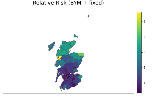
Fixed effects summary (β and 95 CI)
Interpreting fixed effects is easy in a log‑link Poisson GLM:
exp(β₀) is the baseline relative risk when AFF=0 and random effects are zero.
exp(β_aff) is the multiplicative change in RR per unit increase in AFF (here AFF is a fraction; e.g. +0.10 = +10 percentage points). Larger positive β_aff means higher RR in districts with greater AFF.
The code below simply extracts the fixed‑effects block and reports estimates and approximate 95% intervals.
n_fixed = comp.meta.n_fixed
n_cols = size(comp.A, 2)
fix_rng = (n_cols - n_fixed + 1):n_cols

β̂_intercept, β̂_aff = mean(post)[fix_rng]
se_intercept, se_aff = std(post)[fix_rng]
z = 1.96  # 95% normal-approx interval
println("Intercept: $(β̂_intercept) ± $(z * se_intercept)")
println("AFF coefficient: $(β̂_aff) ± $(z * se_aff)")
Intercept: -0.2885174556316574 ± 0.32312607537973353
AFF coefficient: 4.818131607643413 ± 3.1475802486195543BYM decomposition: structured vs unstructured effects
Two quick maps help understand “signal vs noise”:
Structured (Besag): smooth, neighbor‑sharing spatial pattern.
Unstructured (IID): local over‑dispersion not explained by smooth structure.
sizes = comp.combined_model.component_sizes
offs = cumsum([0; sizes[1:(end - 1)]])
idx_block(k) = (offs[k] + 1):(offs[k] + sizes[k])
idx_block (generic function with 1 method)Given RHS order here: IID first, Besag second (fixed appended last).
rng_iid = idx_block(1)
rng_besag = idx_block(2)

u_iid = mean(post)[rng_iid]
u_besag = mean(post)[rng_besag]

plt_besag = plot(
    shapes; fill_z = Float64.(u_besag), st = :shape, c = :balance, lc = :gray30,
    legend = false, axis = nothing, aspect_ratio = 1.0,
    title = "Structured effect", cb = :bottom
)
plt_iid = plot(
    shapes; fill_z = Float64.(u_iid), st = :shape, c = :balance, lc = :gray30,
    legend = false, axis = nothing, aspect_ratio = 1.0,
    title = "Unstructured effect", cb = :bottom
)
plot(plt_besag, plt_iid; layout = (1, 2))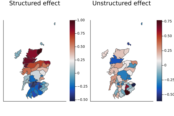
Exceedance probability map: RR greater than 1
A very actionable view: the probability that RR exceeds 1 (i.e., rates are elevated vs expectation). Values near 1 indicate strong evidence for elevation; near 0 suggests lower‑than‑expected; around 0.5 is uncertain.
using Random
N = 2000
rng = Random.MersenneTwister(42)
exceed = zeros(length(df.y))
for _ in 1:N
    x = rand(rng, post)
    ηs = comp.A * x
    exceed .+= (ηs .> 0.0)
end
exceed ./= N

plt_ex = plot(
    shapes; fill_z = reshape(Float64.(exceed), 1, :), st = :shape, c = :viridis, lc = :gray30,
    legend = false, axis = nothing, aspect_ratio = 1.0,
    title = "Exceedance: RR greater than 1", cb = :right
)
plt_ex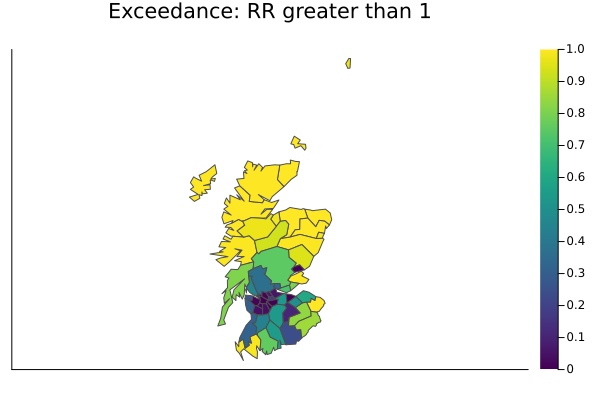
Notes
The
id_to_nodemapping allows using string IDs in the formula; we avoid forcing integer region indices on users.Exposure (E) is supported for Poisson via the
exposure = :Ekeyword inbuild_formula_components.Intrinsic Besag imposes sum-to-zero constraints per connected component.
Isolated islands (with no edges) receive a degenerate prior, such that only the IID part has an effect there.
For more realism, you can tune
τ_besagandτ_iid(orτandφfor BYM2) and add further covariates to the fixed-effects part of the formula.BYM2 is recommended for new analyses: It has more interpretable parameters (τ for overall precision, φ for mixing) and facilitates prior specification. When using BYM2 with an intercept, add
iid_constraint=:sumtozerofor identifiability.
This page was generated using Literate.jl.